Template:Stress-strength analysis

Stress-Strength Analysis

The Expected Probability

Stress-Strength analysis has been used in mechanical component design. The probability of failure is based on the probability of stress exceeding strength. The following equation is used to calculate the expected probability of failure:

[math]\displaystyle{ F=P[Stress\ge Strength]=\int_{0}^{\infty }{{{f}_{Strength}}(x)\cdot {{R}_{Stress}}(x)}dx }[/math]

The expected probability of success or the expected Reliability is calculated as:

[math]\displaystyle{ R=P[Stress\le Strength]=\int_{0}^{\infty }{{{f}_{Stress}}(x)\cdot {{R}_{Strength}}(x)}dx }[/math]

The above calculation assumes both stress and strenght have positive domain. For general cases, the expected reliability can be calcualted using the following equation:

[math]\displaystyle{ R=P[{{X}_{1}}\le {{X}_{2}}]=\frac{1}{{{F}_{1}}(U)-{{F}_{1}}(L)}\int_{L}^{U}{{{f}_{1}}(x)\cdot {{R}_{2}}(x)}dx }[/math]

where:

[math]\displaystyle{ L\le {{X}_{1}}\le U }[/math],

[math]\displaystyle{ \begin{align} & {{X}_{1}}:\text{ Stress; } \\ & {{X}_{2}}:\text{ Strength; } \\ \end{align} }[/math]

When U = infinite and L = 0, the above two equations are the same.

Confidence Interval of the Probability

Both the stress and strenght distributions can be either estimated from actual data or specified by engineers based on engineering knowledge or existing references. Based on the sources of the distribution, there are two types of variations associated with the calculated probability.

Variation in Model Parameters

If both stress and strength distributions are estimated from data sets, then there are uncertainty associated with the estimated distribution parameters. These uncertainty will cause some degree of variation of the calculated probability from the stress-strength analysis. Therefore, we can use these uncertainty to estimate the confidence interval of the calculated probability. To get the confidence interval, we first calcualte the variance of the Reliablility using:

[math]\displaystyle{ Var\left[ R \right]=\int_{0}^{\infty }{Var\left[ {{f}_{1}}(x) \right]}{{\left[ {{R}_{2}}(x) \right]}^{2}}dx+{{\int_{0}^{\infty }{\left[ {{f}_{1}}(x) \right]}}^{2}}Var\left[ {{R}_{2}}(x) \right]dx }[/math]

Variance of [math]\displaystyle{ {{f}_{1}}(x) }[/math] and [math]\displaystyle{ {{R}_{2}}(x) }[/math] can be estimated from the Fisher Information Matrix. For detail, please see chapter Confidence Bounds.

Once the variance of the expected reliability is obtained, the two-sided confidence interval of it can be calcualted using:

[math]\displaystyle{ [\frac{R}{R+(1-R)w},\frac{R}{R+(1-R)/w}] }[/math]

where:

CL is the confidence level;

[math]\displaystyle{ \alpha }[/math] = 1-CL;

[math]\displaystyle{ w=\exp \{{{z}_{1-\alpha /2}}\sqrt{Var(R)}/[R(1-R)]\} }[/math];

[math]\displaystyle{ {{Z}_{1-\alpha /2}} }[/math] is the [math]\displaystyle{ 1-\alpha/2 }[/math] percential of a standard normal distribution.

If the upper bound (U) and lower bound (L) not infinite and 0, the above calcualted variance of R is adjusted by [math]\displaystyle{ {{\left[ {1}/{\left( {{F}_{1}}(U)-{{F}_{1}}(L) \right)}\; \right]}^{2}} }[/math].

Variation in Probability Values

Assume the distributions for stress and strength are known. From the stress-strength equation:

[math]\displaystyle{ R=P[Stress\le Strength]=\int_{0}^{\infty }{{{f}_{Stress}}(x)\cdot {{R}_{Strength}}(x)}dx }[/math]

we know, the calcualted reliability is the Expected value of the probability that a strength value is larger than a stress value. Since both strength and stress are random variables from their distributions, the reliability is also a random variable. This can be explained using the following exampe. Let's first assume stress is a fixed value of 567. The reliability then is:

[math]\displaystyle{ R(567)=\Pr (Strength\gt 567)={{R}_{2}}(567) }[/math]

This is the reliability when the stress value is 567 and when the strength distribution is given. If stress is not a fixed value, instead it follows a distribution, then it can take values other than 567. For instance, it can be a value of 700. Therefore, we get another reliability value of [math]\displaystyle{ {R}(700) }[/math]. Since stress is a random variable, for any stress value [math]\displaystyle{ {x}_{i} }[/math], there is a reliability value of [math]\displaystyle{ R({{x}_{i}}) }[/math] calculated from the strength distribution. We will end up with many [math]\displaystyle{ R({{x}_{i}}) }[/math]s. From these [math]\displaystyle{ R({{x}_{i}}) }[/math]s, we can get its mean and variance. In fact, its mean is the the result from:

[math]\displaystyle{ R=P[Stress\le Strength]=\int_{0}^{\infty }{{{f}_{Stress}}(x)\cdot {{R}_{Strength}}(x)}dx }[/math]

and its variacne is:

[math]\displaystyle{ \begin{align} & Var\left[ R \right]=E\left[ {{R}_{2}}{{\left( {{X}_{1}} \right)}^{2}} \right]-{{\left( E\left[ {{R}_{2}}\left( {{X}_{1}} \right) \right] \right)}^{2}} \\ & =\int_{0}^{\infty }{{{f}_{1}}(x){{\left[ {{R}_{2}}(x) \right]}^{2}}dx}-{{\left( E\left[ {{R}_{2}}\left( {{X}_{1}} \right) \right] \right)}^{2}} \\ & =\int_{0}^{\infty }{{{f}_{1}}(x){{\left[ {{R}_{2}}(x) \right]}^{2}}dx}-{{\left( R \right)}^{2}} \\ \end{align} }[/math]

where R is the expected value of the reliability.

Once the variance of the expected reliability is obtained, the two-sided confidence interval of it can be calcualted using:

[math]\displaystyle{ [\frac{R}{R+(1-R)w},\frac{R}{R+(1-R)/w}] }[/math]

where:

CL is the confidence level;

[math]\displaystyle{ \alpha }[/math] = 1-CL;

[math]\displaystyle{ w=\exp \{{{z}_{1-\alpha /2}}\sqrt{Var(R)}/[R(1-R)]\} }[/math];

[math]\displaystyle{ {{Z}_{1-\alpha /2}} }[/math] is the [math]\displaystyle{ 1-\alpha/2 }[/math] percential of a standard normal distribution.

If the upper bound (U) and lower bound (L) not infinite and 0, the above calcualted variance of R is adjusted by [math]\displaystyle{ {{\left[ {1}/{\left( {{F}_{1}}(U)-{{F}_{1}}(L) \right)}\; \right]}^{2}} }[/math].

Stress-Strength Analysis in Design For Reliability

Weibull++'s Stress-Strength Wizard allows you to perform such calculations.

The Stress-Strength Calculator is accessible from the Tools folder of the Project Explorer. The tool first asks for the locations of the stress and strength data from among the folios available, as shown below.

File:Firstchoice.jpg

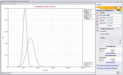
Once the tool knows where to find data for stress and strength, it automatically calculates the reliability and graphs the distributions of the stress and strength data, as shown below.

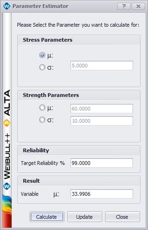
Once the reliability has been calculated, the user has two different options for performing sensitivity analysis (seeing how the system performance changes with changes in parameter values). The user can manually alter the distribution parameters used to calculate the reliability by clicking the “Alter Parameters” link for the appropriate distribution, or the user can use the Parameter Estimator to find what parameters result in a specified target reliability. The “Alter Parameters” link allows the user to manually set what she would like the distribution parameter(s) to be. Alternatively, the Parameter Estimator utility allows the user to select a target reliability to reach and a distribution parameter to adjust. The utility then adjusts the parameter value until the specified target is reached and outputs the parameter value that does so, as shown below.