Template:Difference detection matrix: Difference between revisions
| Line 1: | Line 1: | ||
==Test Design Using Life Difference Detection Matrix== | ==Test Design Using Life Difference Detection Matrix== | ||
The Difference Detection Matrix | Often times, engineers need to design tests for detecting the life differences between two or more product designs. The questions are how many samples and how long the test should be conducted in order to detect a certain amount of difference. There is no simple answer. Usually, advanced design of experiments (DOE) techiques can be utilized. For simple case, such as comparing two designs, the Difference Detection Matrix can be used. The difference detection matrix graphically indicates the amount of test time required to detect a statistically difference in the lives of two populations. | ||
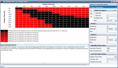
As discussed in the test design using expected failure tiimes plot, if the sample size is know, the failure time of each sample can be obtained based on the assumed failure distribution. With these failure times, we can estimate the failure distribution and any reliability metrics. This process is similar to the simulation used in [[Simumatic]]. This is also the The Difference Detection Matrix takes as inputs information about the samples and information about the testing setup. For each sample, the Difference Detection Matrix needs the size of the sample, the distribution to be assumed for the sample population’s life, and a parameter affecting the variance of each population’s life distribution (e.g., beta for Weibull, and sigma for Normal and Lognormal). The Difference Detection Matrix also needs to know what the maximum allowable test time is, and by what amount of time to increment to the mean lives to be compared. For example, in the design shown below, the mean lives are incremented by 300, up to a mean life of 3000. | |||
Revision as of 23:21, 23 February 2012
Test Design Using Life Difference Detection Matrix
Often times, engineers need to design tests for detecting the life differences between two or more product designs. The questions are how many samples and how long the test should be conducted in order to detect a certain amount of difference. There is no simple answer. Usually, advanced design of experiments (DOE) techiques can be utilized. For simple case, such as comparing two designs, the Difference Detection Matrix can be used. The difference detection matrix graphically indicates the amount of test time required to detect a statistically difference in the lives of two populations.
As discussed in the test design using expected failure tiimes plot, if the sample size is know, the failure time of each sample can be obtained based on the assumed failure distribution. With these failure times, we can estimate the failure distribution and any reliability metrics. This process is similar to the simulation used in Simumatic. This is also the The Difference Detection Matrix takes as inputs information about the samples and information about the testing setup. For each sample, the Difference Detection Matrix needs the size of the sample, the distribution to be assumed for the sample population’s life, and a parameter affecting the variance of each population’s life distribution (e.g., beta for Weibull, and sigma for Normal and Lognormal). The Difference Detection Matrix also needs to know what the maximum allowable test time is, and by what amount of time to increment to the mean lives to be compared. For example, in the design shown below, the mean lives are incremented by 300, up to a mean life of 3000.

The last thing the Difference Detection Matrix needs is what amounts of testing are available. The lengths of testing are initialized automatically, but can easily be modified by simply clicking on the pulldown menu and entering the time desired. When you are ready to calculate new values, just press the calculate icon in the right-hand panel.
After matrix values have been calculated, their codes can be interpreted using the legend below the matrix. The legend shows what level of testing corresponds to each color and code. In the figure shown above, a mean life of design 1 of 900 hours can be told from a mean life of design 2 of 1800 hours after 1500 hours of testing (code 3). A black cell indicates that a statistically significant difference between the two populations’ mean lives cannot be detected with the resources available, either due to insufficient sample sizes or inadequate test time.