Template:Expected failure time plots

Test Design Using Expected Failure Time Plots

Test duration is one of the key factors considered in designing a test. If the expected test duration can be estimated ahead of the test, test resources can be better allocated. In this section, we will explain how to estimated the expected test time based on test sample size and the assumed underlying failure distribution.

The EFTC tool works by first calculating the probability of failure F as a function of the sample size n and number of failures r. This function is given by the equation [math]\displaystyle{ f\left(n,r,CL\right)=\frac{1}{1+\frac{n-r+1}{rF_{2r,2\left(n-r+1\right),1-CL}}} }[/math] where CL is the confidence level.

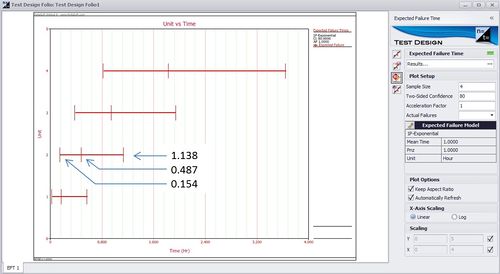
For example, given n = 4, r = 2 and CL = 0.5, the median rank for F is [math]\displaystyle{ f\left(4,2,0.5\right)=\frac{1}{1+\frac{4-2+1}{2F_{4,2\left(3\right),0.5}}}=0.385728 }[/math] The 80% 2-sided confidence interval on the probability of failure F is bounded by [math]\displaystyle{ f\left(4,2,0.1\right)=\frac{1}{1+\frac{4-2+1}{2F_{4,2\left(3\right),0.9}}}=0.142559 }[/math] and [math]\displaystyle{ f\left(4,2,0.9\right)=\frac{1}{1+\frac{4-2+1}{2F_{4,2\left(3\right),0.1}}}=0.679539 }[/math] With the probabilities of failure known, and assuming the failure distribution is exponentially distributed with parameter \(\lambda\,\!\) = 1, the expected times to failure can be calculated.

For example, the median time to the second failure is calculated as [math]\displaystyle{ t=-\frac{ln\left(1-F\right)}{\lambda}=-\frac{1-0.385728}{1}=0.48732 }[/math] Similarly, the 10th percentile and 90th percentiles of time to failure are calculated as [math]\displaystyle{ t=-\frac{1-0.142559}{1}=0.153803 }[/math] and [math]\displaystyle{ t=-\frac{1-0.679539}{1}=1.137995 }[/math] The above results can also be seen in Weibull++ as shown below.