Template:Example: Logistic distribution example: Difference between revisions
Jump to navigation
Jump to search
[math]\displaystyle{ \overset{{}}{\mathop{\text{Table 10}\text{.1 - Times-to-Failure Data with Suspensions}}}\, }[/math]
[math]\displaystyle{ \begin{matrix}
\text{Data Point Index} & \text{State F or S} & \text{State End Time} \\
\text{1} & \text{F} & \text{8} \\
\text{2} & \text{F} & \text{10} \\
\text{3} & \text{F} & \text{15} \\
\text{4} & \text{F} & \text{17} \\
\text{5} & \text{F} & \text{19} \\
\text{6} & \text{F} & \text{26} \\
\text{7} & \text{F} & \text{27} \\
\text{8} & \text{S} & \text{28} \\
\text{9} & \text{S} & \text{28} \\
\text{10} & \text{S} & \text{28} \\
\end{matrix} }[/math]
No edit summary |
|
(No difference)
| |
Revision as of 22:49, 14 February 2012
A Logistic Distribution Example
The lifetime of a mechanical valve is known to follow a logistic distribution. Ten units were tested for 28 months and the following months-to-failure data was collected.
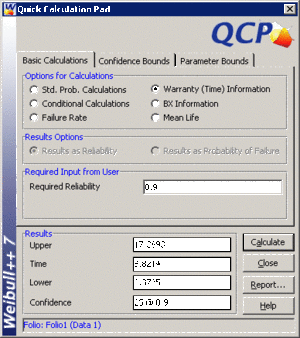
- • Determine the valve's design life if specifications call for a reliability goal of 0.90.
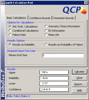
- • The valve is to be used in a pumping device that requires 1 month of continuous operation. What is the probability of the pump failing due to the valve?
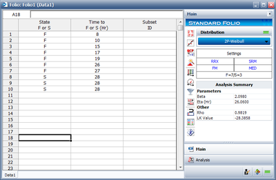
This data set can be entered into Weibull++ as follows:
The computed parameters for maximum likelihood are:
- [math]\displaystyle{ \begin{align} & \widehat{\mu }= & 22.34 \\ & \hat{\sigma }= & 6.15 \end{align} }[/math]
- • The valve's design life, along with 90% two sided confidence bounds, can be obtained using the QCP as follows:
- • The probability, along with 90% two sided confidence bounds, that the pump fails due to a valve failure during the first month is obtained as follows:


