Template:Logistic probability paper: Difference between revisions
(Created page with '====Probability Paper==== The form of the Logistic probability paper is based on linearizing the <math>cdf</math> . From Eqn. (UnR fcn), <math>z</math> can be calculated as a…') |
|||
| Line 1: | Line 1: | ||
== | ==Logistic Distribution Probability Paper== | ||
The form of the Logistic probability paper is based on linearizing the <math>cdf</math> . | The form of the Logistic probability paper is based on linearizing the <math>cdf</math> . | ||
From Eqn. (UnR fcn), <math>z</math> can be calculated as a function of the <math>cdf</math> <math>F</math> as follows: | From Eqn. (UnR fcn), <math>z</math> can be calculated as a function of the <math>cdf</math> <math>F</math> as follows: | ||
Revision as of 22:45, 14 February 2012
Logistic Distribution Probability Paper
The form of the Logistic probability paper is based on linearizing the [math]\displaystyle{ cdf }[/math] . From Eqn. (UnR fcn), [math]\displaystyle{ z }[/math] can be calculated as a function of the [math]\displaystyle{ cdf }[/math] [math]\displaystyle{ F }[/math] as follows:
- [math]\displaystyle{ z=\ln (F)-\ln (1-F) }[/math]
or using Eqn. (z func of parameters)
- [math]\displaystyle{ \frac{T-\mu }{\sigma }=\ln (F)-\ln (1-F) }[/math]
- Then:
- [math]\displaystyle{ \ln (F)-\ln (1-F)=-\frac{\mu }{\sigma }+\frac{1}{\sigma }T }[/math]
- Now let:
- [math]\displaystyle{ y=\ln (F)-\ln (1-F) }[/math]
- [math]\displaystyle{ x=T }[/math]
- and:
- [math]\displaystyle{ a=-\frac{\mu }{\sigma } }[/math]
- [math]\displaystyle{ b=\frac{1}{\sigma } }[/math]
which results in the following linear equation:
- [math]\displaystyle{ y=a+bx }[/math]
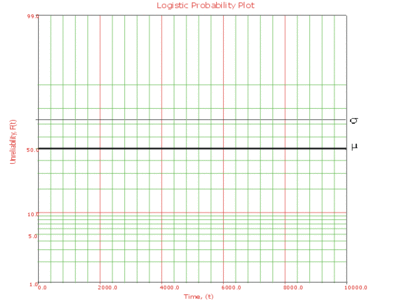
The logistic probability paper resulting from this linearized [math]\displaystyle{ cdf }[/math] function is shown next.
Since the logistic distribution is symmetrical, the area under the [math]\displaystyle{ pdf }[/math] curve from [math]\displaystyle{ -\infty }[/math] to [math]\displaystyle{ \mu }[/math] is [math]\displaystyle{ 0.5 }[/math] , as is the area from [math]\displaystyle{ \mu }[/math] to [math]\displaystyle{ +\infty }[/math] . Consequently, the value of [math]\displaystyle{ \mu }[/math] is said to be the point where [math]\displaystyle{ R(t)=Q(t)=50% }[/math] . This means that the estimate of [math]\displaystyle{ \mu }[/math] can be read from the point where the plotted line crosses the 50% unreliability line.
For [math]\displaystyle{ z=1 }[/math] , [math]\displaystyle{ \sigma =t-\mu }[/math] and [math]\displaystyle{ R(t)=\tfrac{1}{1+\exp (1)}\approx 0.2689. }[/math] Therefore, [math]\displaystyle{ \sigma }[/math] can be found by subtracting [math]\displaystyle{ \mu }[/math] from the time value where the plotted probability line crosses the 73.10% unreliability (26.89% reliability) horizontal line.
