Template:Example: Lognormal Distribution RRY

Lognormal Distribution RRY Example

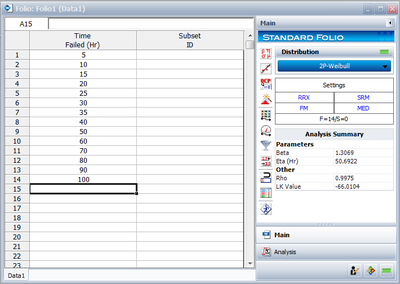
Fourteen units were reliability tested and the following life test data were obtained:

Table 9.1 - Life Test Data for Example 2
Data point index	Time-to-failure
1	5
2	10
3	15
4	20
5	25
6	30
7	35
8	40
9	50
10	60
11	70
12	80
13	90
14	100

Assuming the data follow a lognormal distribution, estimate the parameters and the correlation coefficient, [math]\displaystyle{ \rho }[/math] , using rank regression on Y.

Solution Construct Table 9.2, as shown next.

[math]\displaystyle{ \overset{{}}{\mathop{\text{Table 9}\text{.2 - Least Squares Analysis}}}\, }[/math] [math]\displaystyle{ \begin{matrix} N & T_{i} & F(T_{i}) & {T_{i}}'& y_{i} & {{T_{i}}'}^{2} & y_{i}^{2} & T_{i} y_{i} \\ \text{1} & \text{5} & \text{0}\text{.0483} & \text{1}\text{.6094}& \text{-1}\text{.6619} & \text{2}\text{.5903} & \text{2}\text{.7619} & \text{-2}\text{.6747} \\ \text{2} & \text{10} & \text{0}\text{.1170} & \text{2.3026}& \text{-1.1901} & \text{5.3019} & \text{1.4163} & \text{-2.7403} \\ \text{3} & \text{15} & \text{0}\text{.1865} & \text{2.7080}&\text{-0.8908} & \text{7.3335} & \text{0.7935} & \text{-2.4123} \\ \text{4} & \text{20} & \text{0}\text{.2561} & \text{2.9957} &\text{-0.6552} & \text{8.9744} & \text{0.4292} & \text{-1.9627} \\ \text{5} & \text{25} & \text{0}\text{.3258} & \text{3.2189}& \text{-0.4512} & \text{10.3612} & \text{0.2036} & \text{-1.4524} \\ \text{6} & \text{30} & \text{0}\text{.3954} & \text{3.4012}& \text{-0.2647} & \text{11.5681} & \text{0.0701} & \text{-0.9004} \\ \text{7} & \text{35} & \text{0}\text{.4651} & \text{3.5553} & \text{-0.0873} & \text{12.6405} & \text{-0.0076}& \text{-0.3102} \\ \text{8} & \text{40} & \text{0}\text{.5349} & \text{3.6889}& \text{0.0873} & \text{13.6078} & \text{0.0076} & \text{0.3219} \\ \text{9} & \text{50} & \text{0}\text{.6046} & \text{3.912} & \text{0.2647} & \text{15.3039} & \text{0.0701} &\text{1.0357} \\ \text{10} & \text{60} & \text{0}\text{.6742} & \text{4.0943} & \text{0.4512} & \text{16.7637} & \text{0.2036}&\text{1.8474} \\ \text{11} & \text{70} & \text{0}\text{.7439} & \text{4.2485} & \text{0.6552} & \text{18.0497}& \text{0.4292} & \text{2.7834} \\ \text{12} & \text{80} & \text{0}\text{.8135} & \text{4.382} & \text{0.8908} & \text{19.2022} & \text{0.7935} & \text{3.9035} \\ \text{13} & \text{90} & \text{0}\text{.8830} & \text{4.4998} & \text{1.1901} & \text{20.2483}&\text{1.4163} & \text{5.3552} \\ \text{14} & \text{100}& \text{1.9517} & \text{4.6052} & \text{1.6619} & \text{21.2076} &\text{2.7619} & \text{7.6533} \\ \sum_{}^{} & \text{ } & \text{ } & \text{49.222} & \text{0} & \text{183.1531} & \text{11.3646} & \text{10.4473} \\ \end{matrix} }[/math]

The median rank values ( [math]\displaystyle{ F({{T}_{i}}) }[/math] ) can be found in rank tables or by using the Quick Statistical Reference in Weibull++ .

The [math]\displaystyle{ {{y}_{i}} }[/math] values were obtained from the standardized normal distribution's area tables by entering for [math]\displaystyle{ F(z) }[/math] and getting the corresponding [math]\displaystyle{ z }[/math] value ( [math]\displaystyle{ {{y}_{i}} }[/math] ).

Given the values in the table above, calculate [math]\displaystyle{ \widehat{a} }[/math] and [math]\displaystyle{ \widehat{b} }[/math] using Eqns. (aaln) and (bbln):

[math]\displaystyle{ \begin{align} & \widehat{b}= & \frac{\underset{i=1}{\overset{14}{\mathop{\sum }}}\,T_{i}^{\prime }{{y}_{i}}-(\underset{i=1}{\overset{14}{\mathop{\sum }}}\,T_{i}^{\prime })(\underset{i=1}{\overset{14}{\mathop{\sum }}}\,{{y}_{i}})/14}{\underset{i=1}{\overset{14}{\mathop{\sum }}}\,T_{i}^{\prime 2}-{{(\underset{i=1}{\overset{14}{\mathop{\sum }}}\,T_{i}^{\prime })}^{2}}/14} \\ & & \\ & \widehat{b}= & \frac{10.4473-(49.2220)(0)/14}{183.1530-{{(49.2220)}^{2}}/14} \end{align} }[/math]

or:

[math]\displaystyle{ \widehat{b}=1.0349 }[/math]

and:

[math]\displaystyle{ \widehat{a}=\frac{\underset{i=1}{\overset{N}{\mathop{\sum }}}\,{{y}_{i}}}{N}-\widehat{b}\frac{\underset{i=1}{\overset{N}{\mathop{\sum }}}\,T_{i}^{\prime }}{N} }[/math]

or:

[math]\displaystyle{ \widehat{a}=\frac{0}{14}-(1.0349)\frac{49.2220}{14}=-3.6386 }[/math]

Therefore, from Eqn. (bln):

[math]\displaystyle{ {{\sigma }_{{{T}'}}}=\frac{1}{\widehat{b}}=\frac{1}{1.0349}=0.9663 }[/math]

and from Eqn. (aln):

[math]\displaystyle{ {\mu }'=-\widehat{a}\cdot {{\sigma }_{{{T}'}}}=-(-3.6386)\cdot 0.9663 }[/math]

or:

[math]\displaystyle{ {\mu }'=3.516 }[/math]

The mean and the standard deviation of the lognormal distribution are obtained using Eqns. (mean) and (sdv):

[math]\displaystyle{ \overline{T}=\mu ={{e}^{3.516+\tfrac{1}{2}{{0.9663}^{2}}}}=53.6707\text{ hours} }[/math]

and:

[math]\displaystyle{ {{\sigma }_{T}}=\sqrt{({{e}^{2\cdot 3.516+{{0.9663}^{2}}}})({{e}^{{{0.9663}^{2}}}}-1)}=66.69\text{ hours} }[/math]

The correlation coefficient can be estimated using Eqn. (RHOln):

[math]\displaystyle{ \widehat{\rho }=0.9754 }[/math]

The above example can be repeated using Weibull++ , using RRY.

The mean can be obtained from the QCP and both the mean and the standard deviation can be obtained from the Function Wizard.