Template:Example: Normal Distribution RRY: Difference between revisions
No edit summary |
No edit summary |
||
| Line 109: | Line 109: | ||
:*Click the Calculate icon located on the Main page. | :*Click the Calculate icon located on the Main page. | ||
[[Image: | [[Image:Normal RRY Setting.png|thumb|center|400px| ]] | ||
The probability plot is shown next. | The probability plot is shown next. | ||
[[Image: | [[Image:Normal RRY Plot.png|thumb|center|400px| ]] | ||
Revision as of 21:01, 10 February 2012
Normal Distribution RRY Example
Fourteen units were reliability tested and the following life test data were obtained:
| Table 8.1 -The test data | |
| Data point index | Time-to-failure |
|---|---|
| 1 | 5 |
| 2 | 10 |
| 3 | 15 |
| 4 | 20 |
| 5 | 25 |
| 6 | 30 |
| 7 | 35 |
| 8 | 40 |
| 9 | 50 |
| 10 | 60 |
| 11 | 70 |
| 12 | 80 |
| 13 | 90 |
| 14 | 100 |
Assuming the data follow a normal distribution, estimate the parameters and determine the correlation coefficient, [math]\displaystyle{ \rho }[/math] , using rank regression on Y.
Solution
Construct a table like the one shown next.
- The median rank values ( [math]\displaystyle{ F({{t}_{i}}) }[/math] ) can be found in rank tables, available in many statistical texts, or they can be estimated by using the Quick Statistical Reference in Weibull++.
- The [math]\displaystyle{ {{y}_{i}} }[/math] values were obtained from standardized normal distribution's area tables by entering for [math]\displaystyle{ F(z) }[/math] and getting the corresponding [math]\displaystyle{ z }[/math] value ( [math]\displaystyle{ {{y}_{i}} }[/math] ). As with the median rank values, these standard normal values can be obtained with the Quick Statistical Reference.
Given the values in Table 8.2, calculate [math]\displaystyle{ \widehat{a} }[/math] and [math]\displaystyle{ \widehat{b} }[/math] using:
- [math]\displaystyle{ \begin{align} & \widehat{b}= & \frac{\underset{i=1}{\overset{14}{\mathop{\sum }}}\,{{T}_{i}}{{y}_{i}}-(\underset{i=1}{\overset{14}{\mathop{\sum }}}\,{{T}_{i}})(\underset{i=1}{\overset{14}{\mathop{\sum }}}\,{{y}_{i}})/14}{\underset{i=1}{\overset{14}{\mathop{\sum }}}\,T_{i}^{2}-{{(\underset{i=1}{\overset{14}{\mathop{\sum }}}\,{{T}_{i}})}^{2}}/14} \\ & & \\ & \widehat{b}= & \frac{365.2711-(630)(0)/14}{40,600-{{(630)}^{2}}/14}=0.02982 \end{align} }[/math]
and:
- [math]\displaystyle{ \widehat{a}=\overline{y}-\widehat{b}\overline{T}=\frac{\underset{i=1}{\overset{N}{\mathop{\sum }}}\,{{y}_{i}}}{N}-\widehat{b}\frac{\underset{i=1}{\overset{N}{\mathop{\sum }}}\,{{t}_{i}}}{N} }[/math]
or:
- [math]\displaystyle{ \widehat{a}=\frac{0}{14}-(0.02982)\frac{630}{14}=-1.3419 }[/math]
Therefore:
- [math]\displaystyle{ \widehat{\sigma}=\frac{1}{\hat{b}}=\frac{1}{0.02982}=33.5367 }[/math]
and:
- [math]\displaystyle{ \widehat{\mu }=-\widehat{a}\cdot \widehat{\sigma }=-(-1.3419)\cdot 33.5367\simeq 45 }[/math]
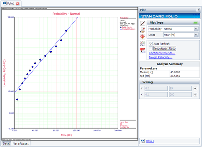
or [math]\displaystyle{ \widehat{\mu }=45 }[/math] hours [math]\displaystyle{ . }[/math]
The correlation coefficient can be estimated using:
- [math]\displaystyle{ \widehat{\rho }=0.979 }[/math]
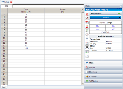
The preceding example can be repeated using Weibull++ .
- Create a new folio for Times-to-Failure data, and enter the data given in Table 8.1.
- Choose Normal from the Distributions list.
- Go to the Analysis page and select Rank Regression on Y (RRY).
- Click the Calculate icon located on the Main page.
The probability plot is shown next.

