Template:ProbabilityDensitynCumulativeDistributionFunctions

The Probability Density and Cumulative Distribution Functions

Designations

From probability and statistics, given a continuous random variable, we denote:

• The probability density function, pdf, as f(x).
• The cumulative distribution function, cdf, as F(x).

The pdf and cdf give a complete description of the probability distribution of a random variable.

Definitions

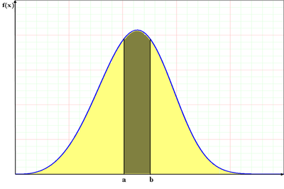
If [math]\displaystyle{ X }[/math] is a continuous random variable, then the probability density function, [math]\displaystyle{ pdf }[/math], of [math]\displaystyle{ X }[/math], is a function [math]\displaystyle{ f(x) }[/math] such that for two numbers, [math]\displaystyle{ a }[/math] and [math]\displaystyle{ b }[/math] with [math]\displaystyle{ a\le b }[/math]:

[math]\displaystyle{ P(a \le X \le b)=\int_a^b f(x)dx }[/math] and [math]\displaystyle{ f(x)\ge 0 }[/math] for all x.

That is, the probability that takes on a value in the interval [a,b] is the area under the density function from [math]\displaystyle{ a }[/math] to [math]\displaystyle{ b }[/math]. The cumulative distribution function, [math]\displaystyle{ cdf }[/math], is a function [math]\displaystyle{ F(x) }[/math] of a random variable, [math]\displaystyle{ X }[/math], and is defined for a number [math]\displaystyle{ x }[/math] by:

[math]\displaystyle{ F(x)=P(X\le x)=\int_0^x f(s)ds }[/math]

That is, for a given value [math]\displaystyle{ x }[/math], [math]\displaystyle{ F(x) }[/math] is the probability that the observed value of [math]\displaystyle{ X }[/math] will be at most [math]\displaystyle{ x }[/math]. Note that the limits of integration depend on the domain of [math]\displaystyle{ f(x) }[/math]. For example, for all the distributions considered in this reference, this domain would be [math]\displaystyle{ [0,+\infty] }[/math], [math]\displaystyle{ [-\infty ,+\infty] }[/math] or [math]\displaystyle{ [\gamma ,+\infty] }[/math]. In the case of [math]\displaystyle{ [\gamma ,+\infty ] }[/math], we use the constant [math]\displaystyle{ \gamma }[/math] to denote an arbitrary non-zero point (or a location that indicates the starting point for the distribution). The next figure illustrates the relationship between the probability density function and the cumulative distribution function.

A graphical representation of the relationship between the pdf and cdf.

Mathematical Relationship Between the [math]\displaystyle{ pdf }[/math] and [math]\displaystyle{ cdf }[/math] The mathematical relationship between the [math]\displaystyle{ pdf }[/math] and [math]\displaystyle{ cdf }[/math] is given by:

[math]\displaystyle{ F(x)=\int_{-\infty }^x f(s)ds }[/math]

Conversely:

[math]\displaystyle{ f(x)=\frac{d(F(x))}{dx} }[/math]

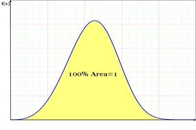
In plain English, the value of the [math]\displaystyle{ cdf }[/math] at [math]\displaystyle{ x }[/math] is the area under the probability density function up to [math]\displaystyle{ x }[/math], if so chosen. It should also be pointed out that the total area under the [math]\displaystyle{ pdf }[/math] is always equal to 1, or mathematically:

[math]\displaystyle{ \int_{-\infty }^{\infty }f(x)dx=1 }[/math]

An example of a probability density function is the well-known normal distribution, whose [math]\displaystyle{ pdf }[/math] is given by:

[math]\displaystyle{ f(t)={\frac{1}{\sigma \sqrt{2\pi }}}{e^{-\frac{1}{2}}(\frac{t-\mu}{\sigma})^2} }[/math]

where [math]\displaystyle{ \mu }[/math] is the mean and [math]\displaystyle{ \sigma }[/math] is the standard deviation. The normal distribution is a two-parameter distribution, i.e. with two parameters [math]\displaystyle{ \mu }[/math] and [math]\displaystyle{ \sigma }[/math]. Another two-parameter distribution is the lognormal distribution, whose [math]\displaystyle{ pdf }[/math] is given by:

[math]\displaystyle{ f(t)=\frac{1}{t\cdot {{\sigma }^{\prime }}\sqrt{2\pi }}{e}^{-\tfrac{1}{2}(\tfrac{t^{\prime}-{\mu^{\prime}}}{\sigma^{\prime}})^2} }[/math]

where [math]\displaystyle{ t^{\prime} }[/math] is the natural logarithm of the times-to-failure, [math]\displaystyle{ \mu^{\prime} }[/math] is the mean of the natural logarithms of the times-to-failure and [math]\displaystyle{ \sigma^{\prime} }[/math] is the standard deviation of the natural logarithms of the times-to-failure, [math]\displaystyle{ t^{\prime } }[/math].