Template:The effect of beta on the Weibull pdf

The Effect of β on the [math]\displaystyle{ pdf }[/math]

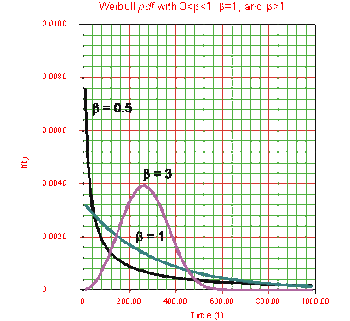
Figure 6-1 shows the effect of different values of the shape parameter, β, on the shape of the [math]\displaystyle{ pdf }[/math]. One can see that the shape of the can take on a variety of forms based on the value of β.

Figure 6-1: The effect of the Weibull shape parameter on the [math]\displaystyle{ pdf }[/math].

For [math]\displaystyle{ 0\lt \beta \leq 1 }[/math]:

• As t→0 (or γ), f(T)→∞.
• As T→∞, f(t)→0.
• f(t) decreases monotonically and is convex as increases beyond the value of γ.
• The mode is non-existent.

For β > 1:

• f(t) = 0 at (or γ).
• f(t) increases as [math]\displaystyle{ t\rightarrow \tilde{T} }[/math] (the mode) and decreases thereafter.
• For β < 2.6 the Weibull [math]\displaystyle{ pdf }[/math] is positively skewed (has a right tail), for 2.6 < β < 3.7 its coefficient of skewness approaches zero (no tail). Consequently, it may approximate the normal [math]\displaystyle{ pdf }[/math] , and for β > 3.7 it is negatively skewed (left tail). The way the value of β relates to the physical behavior of the items being modeled becomes more apparent when we observe how its different values affect the reliability and failure rate functions. Note that for β = 0.999, f(0) = ∞, but for β = 1.001, f(0) = 0. This abrupt shift is what complicates MLE estimation when β is close to one.