Template:Example: 2P Weibull Distribution RRY: Difference between revisions
(Created page with '==== 2P Weibull Distribution Example ==== Consider the data in Example 1, where six units were tested to failure and the following failure times were recorded: 16, 34, 53, 75, 93…') |
No edit summary |
||
| Line 2: | Line 2: | ||
Consider the data in Example 1, where six units were tested to failure and the following failure times were recorded: 16, 34, 53, 75, 93 and 120 hours. Estimate the parameters and the correlation coefficient using rank regression on Y, assuming that the data follow the two-parameter Weibull distribution. | Consider the data in Example 1, where six units were tested to failure and the following failure times were recorded: 16, 34, 53, 75, 93 and 120 hours. Estimate the parameters and the correlation coefficient using rank regression on Y, assuming that the data follow the two-parameter Weibull distribution. | ||
'''Solution''' | |||
Construct a table as shown below. | Construct a table as shown below. | ||
{|align="center" border=1 cellspacing=1 | {|align="center" border=1 cellspacing=1 | ||
|- | |- | ||
|colspan="8" style="text-align:center"| Table | |colspan="8" style="text-align:center"| Table 8.1 - Least Squares Analysis | ||
|- | |- | ||
!<math>N</math> | !<math>N</math> | ||
| Line 34: | Line 35: | ||
Utilizing the values from Table | Utilizing the values from Table 8.1, calculate <math> \hat{a} </math> and <math> \hat{b} </math> using the following equations: | ||
::<math> \hat{b} =\frac{\sum\limits_{i=1}^{6}(\ln | ::<math> \hat{b} =\frac{\sum\limits_{i=1}^{6}(\ln t_{i})y_{i}-(\sum\limits_{i=1}^{6}\ln t_{i})(\sum\limits_{i=1}^{6}y_{i})/6}{ \sum\limits_{i=1}^{6}(\ln t_{i})^{2}-(\sum\limits_{i=1}^{6}\ln t_{i})^{2}/6} | ||
</math> | </math> | ||
::<math> \hat{b}=\frac{-8.0699-(23.9068)(-3.0070)/6}{97.9909-(23.9068)^{2}/6} </math> | ::<math> \hat{b}=\frac{-8.0699-(23.9068)(-3.0070)/6}{97.9909-(23.9068)^{2}/6} </math> | ||
or | |||
::<math> \hat{b}=1.4301 </math> | ::<math> \hat{b}=1.4301 </math> | ||
and: | |||
::<math> \hat{a}=\overline{y}-\hat{b}\overline{T}=\frac{\sum \limits_{i=1}^{N}y_{i}}{N}-\hat{b}\frac{\sum\limits_{i=1}^{N}\ln | ::<math> \hat{a}=\overline{y}-\hat{b}\overline{T}=\frac{\sum \limits_{i=1}^{N}y_{i}}{N}-\hat{b}\frac{\sum\limits_{i=1}^{N}\ln t_{i}}{N } </math> | ||
:or: | :or: | ||
| Line 52: | Line 53: | ||
::<math> \hat{a}=\frac{(-3.0070)}{6}-(1.4301)\frac{23.9068}{6}=-6.19935 </math> | ::<math> \hat{a}=\frac{(-3.0070)}{6}-(1.4301)\frac{23.9068}{6}=-6.19935 </math> | ||
Therefore | Therefore: | ||
::<math> \hat{\beta }=\hat{b}=1.4301 </math> | ::<math> \hat{\beta }=\hat{b}=1.4301 </math> | ||
and | and: | ||
::<math> \hat{\eta }=e^{-\frac{\hat{a}}{\hat{b}}}=e^{-\frac{(-6.19935)}{ 1.4301}} </math> | ::<math> \hat{\eta }=e^{-\frac{\hat{a}}{\hat{b}}}=e^{-\frac{(-6.19935)}{ 1.4301}} </math> | ||
or: | |||
::<math> \hat{\eta }=76.318\text{ hr} </math> | ::<math> \hat{\eta }=76.318\text{ hr} </math> | ||
The correlation coefficient can be estimated | The correlation coefficient can be estimated as: | ||
::<math> \hat{\rho }=0.9956 </math> | ::<math> \hat{\rho }=0.9956 </math> | ||
| Line 117: | Line 118: | ||
If desired, the Weibull <math>pdf</math> representing these data can be written as: | If desired, the Weibull <math>pdf</math> representing these data can be written as: | ||
::<math> f( | ::<math> f(t)={\frac{\beta }{\eta }}\left( {\frac{t}{\eta }}\right) ^{\beta -1}e^{-\left( {\frac{t}{\eta }}\right) ^{\beta }} </math> | ||
:or: | :or: | ||
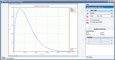
::<math> f( | ::<math> f(t)={\frac{1.4302}{76.317}}\left( {\frac{t}{76.317}}\right) ^{0.4302}e^{-\left( {\frac{t}{76.317}}\right) ^{1.4302}} </math> You can also plot the Weibull by selecting ''Pdf Plot'' from the ''Plot Type'' drop-down menu on the control panel to the right of the plot area. | ||
[[Image:weibullpdffolio16.png|thumb|center|400px]] | [[Image:weibullpdffolio16.png|thumb|center|400px]] | ||
From this point on, different results, reports and plots can be obtained. | From this point on, different results, reports and plots can be obtained. | ||
Revision as of 17:13, 9 February 2012
2P Weibull Distribution Example
Consider the data in Example 1, where six units were tested to failure and the following failure times were recorded: 16, 34, 53, 75, 93 and 120 hours. Estimate the parameters and the correlation coefficient using rank regression on Y, assuming that the data follow the two-parameter Weibull distribution.
Solution
Construct a table as shown below.
| Table 8.1 - Least Squares Analysis | |||||||
| [math]\displaystyle{ N }[/math] | [math]\displaystyle{ T_{i} }[/math] | [math]\displaystyle{ ln(T_{i}) }[/math] | [math]\displaystyle{ F(T_i) }[/math] | [math]\displaystyle{ y_{i} }[/math] | [math]\displaystyle{ (ln{T_i})^2 }[/math] | [math]\displaystyle{ {y_i}^2 }[/math] | [math]\displaystyle{ (ln{T_i})y_i }[/math] |
|---|---|---|---|---|---|---|---|
| 1 | 16 | 2.7726 | 0.1091 | -2.1583 | 7.6873 | 4.6582 | -5.9840 |
| 2 | 34 | 3.5264 | 0.2645 | -1.1802 | 12.4352 | 1.393 | -4.1620 |
| 3 | 53 | 3.9703 | 0.4214 | -0.6030 | 15.7632 | 0.3637 | -2.3943 |
| 4 | 75 | 4.3175 | 0.5786 | -0.146 | 18.6407 | 0.0213 | -0.6303 |
| 5 | 93 | 4.5326 | 0.7355 | 0.2851 | 20.5445 | 0.0813 | 1.2923 |
| 6 | 120 | 4.7875 | 0.8909 | 0.7955 | 22.9201 | 0.6328 | 3.8083 |
| [math]\displaystyle{ \sum }[/math] | 23.9068 | -3.007 | 97.9909 | 7.1502 | -8.0699 | ||
Utilizing the values from Table 8.1, calculate [math]\displaystyle{ \hat{a} }[/math] and [math]\displaystyle{ \hat{b} }[/math] using the following equations:
- [math]\displaystyle{ \hat{b} =\frac{\sum\limits_{i=1}^{6}(\ln t_{i})y_{i}-(\sum\limits_{i=1}^{6}\ln t_{i})(\sum\limits_{i=1}^{6}y_{i})/6}{ \sum\limits_{i=1}^{6}(\ln t_{i})^{2}-(\sum\limits_{i=1}^{6}\ln t_{i})^{2}/6} }[/math]
- [math]\displaystyle{ \hat{b}=\frac{-8.0699-(23.9068)(-3.0070)/6}{97.9909-(23.9068)^{2}/6} }[/math]
or
- [math]\displaystyle{ \hat{b}=1.4301 }[/math]
and:
- [math]\displaystyle{ \hat{a}=\overline{y}-\hat{b}\overline{T}=\frac{\sum \limits_{i=1}^{N}y_{i}}{N}-\hat{b}\frac{\sum\limits_{i=1}^{N}\ln t_{i}}{N } }[/math]
- or:
- [math]\displaystyle{ \hat{a}=\frac{(-3.0070)}{6}-(1.4301)\frac{23.9068}{6}=-6.19935 }[/math]
Therefore:
- [math]\displaystyle{ \hat{\beta }=\hat{b}=1.4301 }[/math]
and:
- [math]\displaystyle{ \hat{\eta }=e^{-\frac{\hat{a}}{\hat{b}}}=e^{-\frac{(-6.19935)}{ 1.4301}} }[/math]
or:
- [math]\displaystyle{ \hat{\eta }=76.318\text{ hr} }[/math]
The correlation coefficient can be estimated as:
- [math]\displaystyle{ \hat{\rho }=0.9956 }[/math]
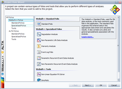
The above example can be repeated using Weibull++. Start Weibull++ and create a new Data Folio.
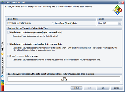
Select the Times-to-failure data option.
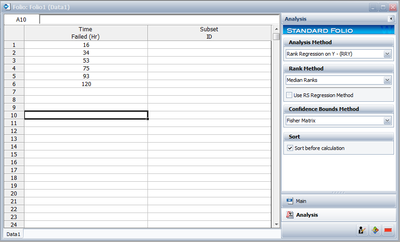
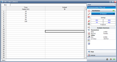
Enter the times-to-failure in the datasheet (ignore the Subset ID column), as shown next. The times-to-failure need not be sorted, Weibull++ will automatically sort the data.
Select the desired method of analysis. Note that we are assuming that the underlying distribution is the Weibull, so make sure that the Weibull distribution is selected. Under Parameters/Type on the Main page, select 2.
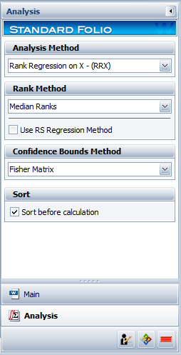
Also, so that you get the same results as this example, switch to the Analysis page and make sure you are using the Rank Regression on Y (RRY) calculation method with this example, as shown next.
Note that this can also be done from the Main page by clicking the left bottom box under the Results area. Each time you click that box you will see the method switch between MLE, RRX, and RRY. Click the Calculate icon,
or select Calculate from the Data menu. The results will appear in the Data Folio's Results area. The next figure shows the results for this example.
You can now plot the results by clicking the Plot icon,
or by selecting Plot Probability from the Data menu.
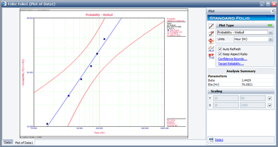
The Weibull probability plot for these data is shown next.
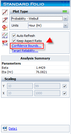
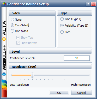
The confidence bounds, as determined from the Fisher matrix, can also be plotted. Select Confidence Bounds from the Plot menu, choose Two-Sided under Sides, Reliability (Type II) under Type and enter 90 for the Confidence level.
The plot will appear as follows,
If desired, the Weibull [math]\displaystyle{ pdf }[/math] representing these data can be written as:
- [math]\displaystyle{ f(t)={\frac{\beta }{\eta }}\left( {\frac{t}{\eta }}\right) ^{\beta -1}e^{-\left( {\frac{t}{\eta }}\right) ^{\beta }} }[/math]
- or:
- [math]\displaystyle{ f(t)={\frac{1.4302}{76.317}}\left( {\frac{t}{76.317}}\right) ^{0.4302}e^{-\left( {\frac{t}{76.317}}\right) ^{1.4302}} }[/math] You can also plot the Weibull by selecting Pdf Plot from the Plot Type drop-down menu on the control panel to the right of the plot area.
From this point on, different results, reports and plots can be obtained.
