Template:One parameter exponential distribution example Probability Plot

Example 1: One Parameter Exponential Example RRY

Six units are put on a life test and tested to failure. The failure times are 7, 12, 19, 29, 41, and 67 hours. Estimate the failure rate parameter for a one-parameter exponential distribution using the probability plotting method.

Solution to Example 1

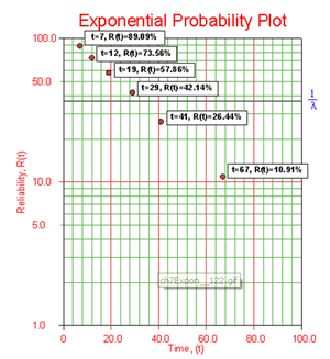
In order to plot the points for the probability plot, the appropriate reliability estimate values must be obtained. These will be equivalent to [math]\displaystyle{ 100%-MR }[/math], since the y-axis represents the reliability and the [math]\displaystyle{ MR }[/math] values represent unreliability estimates.

[math]\displaystyle{ \begin{matrix} \text{Time-to-} & \text{Reliability} \\ \text{failure, hr} & \text{Estimate, }% \\ 7 & 100-10.91=89.09% \\ 12 & 100-26.44=73.56% \\ 19 & 100-42.14=57.86% \\ 29 & 100-57.86=42.14% \\ 41 & 100-73.56=26.44% \\ 67 & 100-89.09=10.91% \\ \end{matrix} }[/math]

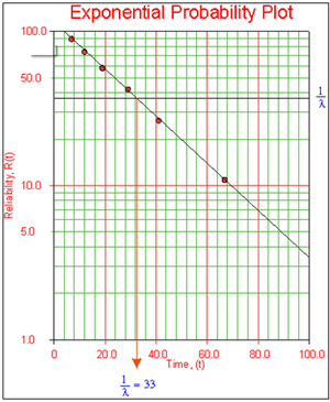
Next, these points are plotted on exponential probability plotting paper. A sample of this type of plotting paper is shown next, with the sample points in place. Notice how these points describe a line with a negative slope. Once the points are plotted, draw the best possible straight line through these points. The time value at which this line intersects with a horizontal line drawn at the 36.8% reliability mark is the mean life, and the reciprocal of this is the failure rate [math]\displaystyle{ \lambda }[/math]. This is because at [math]\displaystyle{ t=m=\tfrac{1}{\lambda } }[/math]:

[math]\displaystyle{ \begin{align} R(t)= & {{e}^{-\lambda \cdot t}} \\ R(t)= & {{e}^{-\lambda \cdot \tfrac{1}{\lambda }}} \\ R(t)= & {{e}^{-1}}=0.368=36.8%. \end{align} }[/math]

These steps are shown graphically in the next pages.

As can be seen in the plot below, the best-fit line through the data points crosses the [math]\displaystyle{ R=36.8% }[/math] line at [math]\displaystyle{ t=33 }[/math] hours.

Since [math]\displaystyle{ \tfrac{1}{\lambda }=33 }[/math] hours, [math]\displaystyle{ \lambda =0.0303 }[/math] failures/hour.