Degradation Data Analysis: Difference between revisions
| Line 77: | Line 77: | ||
<math></math> | <math></math> | ||
[[Image: | [[Image:degradation1.png|thumb|center|400px| ]] | ||
Revision as of 18:21, 27 September 2011
Degradation Analysis
Given that products are more frequently being designed with higher reliability and developed in a shorter amount of time, it is often not possible to test new designs to failure under normal operating conditions. In some cases, it is possible to infer the reliability behavior of unfailed test samples with only the accumulated test time information and assumptions about the distribution. However, this generally leads to a great deal of uncertainty in the results. Another option in this situation is the use of degradation analysis. Degradation analysis involves the measurement and extrapolation of degradation or performance data that can be directly related to the presumed failure of the product in question. Many failure mechanisms can be directly linked to the degradation of part of the product, and degradation analysis allows the user to extrapolate to an assumed failure time based on the measurements of degradation or performance over time.
In some cases, it is possible to directly measure the degradation over time, as with the wear of brake pads or with the propagation of crack size. In other cases, direct measurement of degradation might not be possible without invasive or destructive measurement techniques that would directly affect the subsequent performance of the product. In such cases, the degradation of the product can be estimated through the measurement of certain performance characteristics, such as using resistance to gauge the degradation of a dielectric material. In either case, however, it is necessary to be able to define a level of degradation or performance at which a failure is said to have occurred. With this failure level of performance defined, it is a relatively simple matter to use basic mathematical models to extrapolate the performance measurements over time to the point where the failure is said to occur. Once these have been determined, it is merely a matter of analyzing the extrapolated failure times like conventional time-to-failure data.
Once the level of failure (or the degradation level that would constitute a failure) is defined, the degradation for multiple units over time needs to be measured. As with conventional reliability data, the amount of certainty in the results is directly related to the number of units being tested. The performance or degradation of these units needs to be measured over time, either continuously or at predetermined intervals. Once this information has been recorded, the next task is to extrapolate the performance measurements to the defined failure level in order to estimate the failure time. Weibull++ allows the user to perform such analysis using a linear, exponential, power or logarithmic model to perform this extrapolation. These models have the following forms:
where [math]\displaystyle{ y }[/math] represents the performance, [math]\displaystyle{ x }[/math] represents time, and [math]\displaystyle{ a, }[/math] [math]\displaystyle{ b }[/math] and [math]\displaystyle{ c }[/math] are model parameters to be solved for.
Once the model parameters [math]\displaystyle{ {{a}_{i}} }[/math] , [math]\displaystyle{ {{b}_{i}} }[/math] (and [math]\displaystyle{ {{c}_{i}} }[/math] ) are estimated for each sample [math]\displaystyle{ i }[/math] , a time, [math]\displaystyle{ {{x}_{i}} }[/math] , can be extrapolated, which corresponds to the defined level of failure [math]\displaystyle{ y }[/math] . The computed [math]\displaystyle{ {{x}_{i}} }[/math] values can now be used as our times-to-failure for subsequent life data analysis. As with any sort of extrapolation, one must be careful not to extrapolate too far beyond the actual range of data in order to avoid large inaccuracies (modeling errors).
Example 1
Five turbine blades were tested for crack propagation. The test units are cyclically stressed and inspected every 100,000 cycles for crack length. Failure is defined as a crack of length 30mm or greater.
Following is a table of the test results:
Using degradation analysis with an exponential model for the extrapolation, determine the B10 life for the blades.
Solution to Example 1
The first step is to solve the equation [math]\displaystyle{ y=b\cdot {{e}^{a\cdot x}} }[/math] for [math]\displaystyle{ a }[/math] and [math]\displaystyle{ b }[/math] for each of the test units. Using regression analysis, these values for each of the test units are:
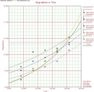
These results are shown graphically in the next figure.
[math]\displaystyle{ }[/math]
These values can now be substituted into the underlying exponential model, solved for [math]\displaystyle{ x }[/math] or:
- [math]\displaystyle{ x=\frac{\text{ln}(y)-\text{ln}(b)}{a} }[/math]
Using the values of [math]\displaystyle{ a }[/math] and [math]\displaystyle{ b }[/math] , with [math]\displaystyle{ y=30 }[/math] , the resulting time at which the crack length reaches 30mm is then found for each sample:
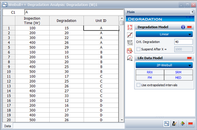
These times-to-failure can now be analyzed in the conventional manner. Assuming a two-parameter Weibull distribution and using the MLE estimation method, the distribution parameters are calculated as [math]\displaystyle{ \beta =8.055 }[/math] and [math]\displaystyle{ \eta =519,555. }[/math] Using these values, the B10 life is calculated to be 392,918 cycles. The degradation analysis tool in Weibull++ performs this type of analysis for you. The following figure shows the data as entered in Weibull++ for this analysis.
[math]\displaystyle{ }[/math]


