Reliability Test Design

Test Design

Quite often, there is a desire to design reliability demonstration tests that have few or no failures. These tests are often required to demonstrate customer reliability and confidence requirements. While it is desirable to be able to test a large population of units to failure in order to obtain information on a product or design's reliability, time and resource constraints sometimes make this impossible. In cases such as these, a test can be run on a specified number of units, or for a specified amount of time, that will demonstrate that the products have met or exceeded a given reliability at a given confidence level. In order to do so without a large amount of cumulative test time or failure data, it is necessary to make assumptions about the failure distribution of the product. In the final analysis, the actual reliability of the units will of course remain unknown, but the reliability engineer will be able to state that certain specifications have been met.

Demonstration Test Design

Frequently, a manufacturer will have to demonstrate that a certain product has met a goal of a certain reliability at a given time with a specific confidence. Often, it will be desired to demonstrate that this goal has been met with a zero-failure test. In order to design and conduct such a test, something about the behavior of the product will need to be known, i.e. the shape parameter of the product's life distribution. Beyond this, nothing more about the test is known, and usually the engineer designing the test will have to study the financial trade-offs between the number of units and amount of test time needed to demonstrate the desired goal. In cases like this, it is useful to have a ``carpet plot that shows the possibilities of how a certain specification can be met.

This methodology requires the use of the cumulative binomial distribution in addition to the assumed distribution of the products' lifetimes. Not only does the life distribution of the products need to be assumed beforehand, but a reasonable assumption of the distribution's shape parameter must be provided as well. Additional information that must be supplied includes the reliability to be demonstrated, the confidence level at which the demonstration takes place, the acceptable number of failures and either the number of available units or the amount of available test time. The output of this analysis can be the amount of time required to test the available units or the required number of units that need to be tested during the available test time.

Reliability Demonstration

Frequently, the entire purpose of designing a test with few or no failures is to demonstrate a certain reliability, [math]\displaystyle{ {{R}_{DEMO}} }[/math] , at a certain time. With the exception of the exponential distribution (and ignoring the location parameter for the time being), this reliability is going to be a function of time, a shape parameter and a scale parameter.

[math]\displaystyle{ {{R}_{DEMO}}=g({{t}_{DEMO}};\theta ,\phi ) }[/math]

where:

[math]\displaystyle{ \begin{align} & & {{t}_{DEMO}}\text{ is the time at which the demonstrated reliability is specified} \\ & & \theta \text{ is the shape parameter} \\ & & \phi \text{ is the scale parameter} \end{align} }[/math]

Since required inputs to the process include [math]\displaystyle{ {{R}_{DEMO}} }[/math] , [math]\displaystyle{ {{t}_{DEMO}} }[/math] and [math]\displaystyle{ \theta }[/math] , the value of the scale parameter can be backed out of the reliability equation of the assumed distribution, and will be used in the calculation of another reliability value, [math]\displaystyle{ {{R}_{TEST}} }[/math] , which is the reliability that is going to be incorporated in the actual test calculation. How this calculation is performed depends on whether one is attempting to solve for the number of units to be tested in an available amount of time, or attempting to find how long to test an available number of test units.

Determining Units for Available Test Time

If one knows that the test is to last a certain amount of time, [math]\displaystyle{ {{t}_{TEST}} }[/math] , the number of units that must be tested to demonstrate the specification must be determined. The first step in accomplishing this involves calculating the [math]\displaystyle{ {{R}_{TEST}} }[/math] value.

This should be a simple procedure since:

[math]\displaystyle{ {{R}_{TEST}}=g({{t}_{TEST}};\theta ,\phi ) }[/math]

and [math]\displaystyle{ {{t}_{DEMO}} }[/math] , [math]\displaystyle{ \theta }[/math] and [math]\displaystyle{ \phi }[/math] are already known, and it is just a matter of plugging these values into the appropriate reliability equation.

We now incorporate a form of the cumulative binomial distribution in order to solve for the required number of units. This form of the cumulative binomial appears as:

[math]\displaystyle{ 1-CL=\underset{i=0}{\overset{f}{\mathop \sum }}\,\frac{n!}{i!\cdot (n-i)!}\cdot {{(1-{{R}_{TEST}})}^{i}}\cdot R_{TEST}^{(n-i)} }[/math]

where:

[math]\displaystyle{ \begin{align} & CL= & \text{the required confidence level} \\ & f= & \text{the allowable number of failures} \\ & n= & \text{the total number of units on test} \\ & {{R}_{TEST}}= & \text{the reliability on test} \end{align} }[/math]

Since [math]\displaystyle{ CL }[/math] and [math]\displaystyle{ f }[/math] are required inputs to the process and [math]\displaystyle{ {{R}_{TEST}} }[/math] has already been calculated, it merely remains to solve the cumulative binomial equation for [math]\displaystyle{ n }[/math] , the number of units that need to be tested.

Determining Test Time for Available Units

The way that one determines the test time for the available number of test units is quite similar to the process described previously. In this case, one knows beforehand the number of units, [math]\displaystyle{ n }[/math] , the number of allowable failures, [math]\displaystyle{ f }[/math] , and the confidence level, [math]\displaystyle{ CL }[/math] . With this information, the next step involves solving Eqn. (relcum) for [math]\displaystyle{ {{R}_{TEST}} }[/math] . With this value known, one can use the appropriate reliability equation to back out the value of [math]\displaystyle{ {{t}_{TEST}} }[/math] , since [math]\displaystyle{ {{R}_{TEST}}=g({{t}_{TEST}};\theta ,\phi ) }[/math] , and [math]\displaystyle{ {{R}_{TEST}} }[/math] , [math]\displaystyle{ \theta }[/math] and [math]\displaystyle{ \phi }[/math] have already been calculated or specified.

MTTF Demonstration

Designing a test to demonstrate a certain value of the [math]\displaystyle{ MTTF }[/math] is identical to designing a reliability demonstration test, with the exception of how the value of the scale parameter [math]\displaystyle{ \phi }[/math] is determined. Given the value of the [math]\displaystyle{ MTTF }[/math] and the value of the shape parameter [math]\displaystyle{ \theta }[/math] , the value of the scale parameter [math]\displaystyle{ \phi }[/math] can be calculated. With this, the analysis can proceed as with the reliability demonstration methodology.

Weibull Distribution Example - Demonstrate Reliability

In this example, we will design a test to demonstrate a reliability of 90% at [math]\displaystyle{ t=100 }[/math] hours, with a 95% confidence. We will assume a Weibull distribution with a shape parameter [math]\displaystyle{ \beta =1.5 }[/math] . No failures will be allowed on this test, or [math]\displaystyle{ f=0 }[/math] .

Determining Units for Available Time

In the above scenario, we know that we have the testing facilities available for [math]\displaystyle{ t=48 }[/math] hours. We must now determine the number of units to test for this amount of time with no failures in order to have demonstrated our reliability goal. The first step is to determine the Weibull scale parameter, [math]\displaystyle{ \eta . }[/math] The Weibull reliability equation is:

[math]\displaystyle{ R={{e}^{-{{(t/\eta )}^{\beta }}}} }[/math]

This can be rewritten as:

[math]\displaystyle{ \eta =\frac{{{t}_{DEMO}}}{{{(-\text{ln}({{R}_{DEMO}}))}^{\tfrac{1}{\beta }}}} }[/math]

Since we know the values of [math]\displaystyle{ {{t}_{DEMO}} }[/math] , [math]\displaystyle{ {{R}_{DEMO}} }[/math] and [math]\displaystyle{ \beta }[/math] , we can substitute these in the equation and solve for [math]\displaystyle{ \eta }[/math] :

[math]\displaystyle{ \eta =\frac{100}{{{(-\text{ln}(0.9))}^{\tfrac{1}{1.5}}}}=448.3 }[/math]

Next, the value of [math]\displaystyle{ {{R}_{TEST}} }[/math] is calculated by:

[math]\displaystyle{ {{R}_{TEST}}={{e}^{-{{({{t}_{TEST}}/\eta )}^{\beta }}}}={{e}^{-{{(48/448.3)}^{1.5}}}}=0.966=96.6%. }[/math]

The last step is to substitute the appropriate values into the cumulative binomial equation, which for the Weibull distribution appears as:

[math]\displaystyle{ 1-C.L.=\underset{i=0}{\overset{f}{\mathop \sum }}\,\frac{n!}{i!\cdot (n-i)!}\cdot {{(1-{{e}^{-{{({{t}_{TEST}}/\eta )}^{\beta }}}})}^{i}}\cdot {{({{e}^{-{{({{t}_{TEST}}/\eta )}^{\beta }}}})}^{(n-i)}} }[/math]

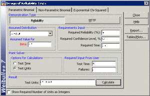
The values of [math]\displaystyle{ CL }[/math] , [math]\displaystyle{ {{t}_{TEST}} }[/math] , [math]\displaystyle{ \beta }[/math] , [math]\displaystyle{ f }[/math] and [math]\displaystyle{ \eta }[/math] have already been calculated or specified, so it merely remains to solve the equation for [math]\displaystyle{ n. }[/math] This value is [math]\displaystyle{ n=85.4994, }[/math] or [math]\displaystyle{ n=86 }[/math] units, since the fractional value must be rounded up to the next integer value. This example solved in Weibull++ is shown next.

Determining Time for Available Units

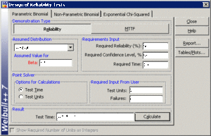
In this case, we will assume that we have 20 units to test, [math]\displaystyle{ n=20 }[/math] , and must determine the test time, [math]\displaystyle{ {{t}_{TEST}}. }[/math] We have already determined the value of the scale parameter, [math]\displaystyle{ \eta }[/math] , in the previous example. Since we know the values of [math]\displaystyle{ n }[/math] , [math]\displaystyle{ CL }[/math] , [math]\displaystyle{ f }[/math] , [math]\displaystyle{ \eta }[/math] and [math]\displaystyle{ \beta }[/math] , it remains to solve Eqn. (weibcum) for [math]\displaystyle{ {{t}_{TEST}} }[/math] . This value is [math]\displaystyle{ {{t}_{TEST}}=126.4339 }[/math] hours. This example solved in Weibull++ is shown next.

Weibull Distribution Example - Demonstrate MTTF

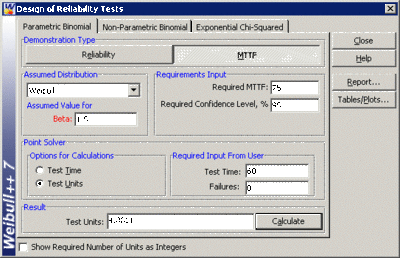
In this example, we will design a test to demonstrate [math]\displaystyle{ MTTF=75 }[/math] hours, with a 95% confidence. We will once again assume a Weibull distribution with a shape parameter [math]\displaystyle{ \beta =1.5 }[/math] . No failures will be allowed on this test, or [math]\displaystyle{ f=0 }[/math] . We want to determine the number of units to test for [math]\displaystyle{ {{t}_{TEST}}=60 }[/math] hours to demonstrate this goal.

The first step in this case involves determining the value of the scale parameter [math]\displaystyle{ \eta }[/math] from the [math]\displaystyle{ MTTF }[/math] equation. The equation for the [math]\displaystyle{ MTTF }[/math] for the Weibull distribution is:

[math]\displaystyle{ MTTF=\eta \cdot \Gamma (1+\frac{1}{\beta }) }[/math]

where [math]\displaystyle{ \Gamma (x) }[/math] is the gamma function of [math]\displaystyle{ x }[/math] . This can be rearranged in terms of .. :

[math]\displaystyle{ \eta =\frac{MTTF}{\Gamma (1+\tfrac{1}{\beta })} }[/math]

Since [math]\displaystyle{ MTTF }[/math] and [math]\displaystyle{ \beta }[/math] have been specified, it is a relatively simple matter to calculate [math]\displaystyle{ \eta =83.1 }[/math] . From this point on, the procedure is the same as the reliability demonstration example. Next, the value of [math]\displaystyle{ {{R}_{TEST}} }[/math] is calculated as:

[math]\displaystyle{ {{R}_{TEST}}={{e}^{-{{({{t}_{TEST}}/\eta )}^{\beta }}}}={{e}^{-{{(60/83.1)}^{1.5}}}}=0.541=54.1% }[/math]

The last step is to substitute the appropriate values into the cumulative binomial equation. The values of [math]\displaystyle{ CL }[/math] , [math]\displaystyle{ {{t}_{TEST}} }[/math] , [math]\displaystyle{ \beta }[/math] , [math]\displaystyle{ f }[/math] and [math]\displaystyle{ \eta }[/math] have already been calculated or specified, so it merely remains to solve Eqn. (relcum) for [math]\displaystyle{ n. }[/math] The value is calculated as [math]\displaystyle{ n=4.8811, }[/math] or [math]\displaystyle{ n=5 }[/math] units, since the fractional value must be rounded up to the next integer value. This example solved in Weibull++ is shown next.

The procedure for determining the required test time proceeds in the same manner, determining [math]\displaystyle{ \eta }[/math] from the [math]\displaystyle{ MTTF }[/math] equation, and following the previously described methodology to determine [math]\displaystyle{ {{t}_{TEST}} }[/math] from Eqn. (weibcum).

Nonparametric Test Design

Eqn. (relcum) can be used for nonparametric demonstration test design. One must merely assume values for three of the inputs of [math]\displaystyle{ CL }[/math] , [math]\displaystyle{ {{R}_{TEST}} }[/math] , [math]\displaystyle{ n }[/math] , and [math]\displaystyle{ f }[/math] , and solve for the fourth. Note that there is no time value associated with this methodology, so one must assume that the value of [math]\displaystyle{ {{R}_{TEST}} }[/math] is associated with the amount of time for which the units were tested.

Constant Failure Rate/Chi-Squared Test Design

Another method for designing tests for products that have an assumed constant failure rate, or exponential life distribution, draws on the chi-squared distribution. These represent the true exponential distribution confidence bounds referred to in Chapter 7. This method only returns the necessary accumulated test time for a demonstrated reliability or [math]\displaystyle{ MTTF }[/math] , not a specific time/test unit combination that is obtained using the cumulative binomial method described above. The accumulated test time is equal to the total amount of time experienced by all of the units on test. Assuming that the units undergo the same amount of test time, this works out to be:

[math]\displaystyle{ {{T}_{a}}=n\cdot {{t}_{TEST}} }[/math]

where [math]\displaystyle{ n }[/math] is the number of units on test and [math]\displaystyle{ {{t}_{TEST}} }[/math] is the test time. The chi-squared equation for test time is:

[math]\displaystyle{ {{T}_{a}}=\frac{MTTF\cdot \chi _{1-CL;2f+2}^{2}}{2} }[/math]

where:

[math]\displaystyle{ \begin{align} & \chi _{1-CL;2f+2}^{2}= & \text{the chi squared distribution} \\ & {{T}_{a}}= & \text{the necessary accumulated test time} \\ & CL= & \text{the confidence level, and} \\ & f= & \text{the number of failures} \end{align} }[/math]

Since this methodology only applies to the exponential distribution, the exponential reliability equation can be rewritten as:

math>MTTF=\frac{t}{-ln(R)}</math>

and substituted into Eqn. (expchi1) for developing a test that demonstrates reliability at a given time, rather than [math]\displaystyle{ MTTF }[/math] :

[math]\displaystyle{ {{T}_{a}}=\frac{\tfrac{{{t}_{DEMO}}}{-ln(R)}\cdot \chi _{1-CL;2f+2}^{2}}{2} }[/math]

Exponential Distribution Example

In this example, we desire to design a test to demonstrate a reliability of 85% at [math]\displaystyle{ {{t}_{DEMO}}=500 }[/math] hours with a 90% confidence, or [math]\displaystyle{ CL=0.9, }[/math] and two allowable failures, [math]\displaystyle{ f=2 }[/math] . The chi-squared value can be determined from tables or the Quick Statistical Reference in Weibull++. In this example, the value is calculated as:

[math]\displaystyle{ \chi _{1-CL;2r+2}^{2}=\chi _{0.1;6}^{2}=10.6446 }[/math]

Substituting this into Eqn. (expchi1), we obtain:

[math]\displaystyle{ {{T}_{a}}=\frac{\tfrac{500}{-ln(0.85)}\cdot 10.6446}{2}=16,374\text{ hours} }[/math]

This means that 16,374 hours of total test time need to be accumulated with two failures in order to demonstrate the specified reliability.

This example solved in Weibull++ is shown next.

Given the test time, one can now solve for the number of units using Eqn. (expchipv1). Similarly, if the number of units is given, one can determine the test time from Eqn. (expchipv1).

SimuMatic

Reliability analysis using simulation, in which reliability analyses are performed a large number of times on data sets that have been created using Monte Carlo simulation, can be a valuable tool for reliability practitioners. Such simulation analyses can assist the analyst to a) better understand life data analysis concepts, b) experiment with the influences of sample sizes and censoring schemes on analysis methods, c) construct simulation-based confidence intervals, d) better understand the concepts behind confidence intervals and e) design reliability tests. This section explores some of the results that can be obtained from simulation analyses with SimuMatic utility in Weibull++.

Parameter Estimation and Confidence Bounds Techniques

In life data analysis, we use data (usually times-to-failure or times-to-success data) obtained from a sample of units to make predictions for the entire population of units. Depending on the sample size, the data censoring scheme and the parameter estimation method, the amount of error in the results can vary widely. To quantify this sampling error, or uncertainty, confidence bounds are widely used. In addition to the analytical calculation methods that are available, simulation can also be used. SimuMatic generates these confidence bounds and assists the practitioner (or the teacher) to visualize and understand them. In addition, it allows the analyst to determine the adequacy of certain parameter estimation methods (such as rank regression on X, rank regression on Y and maximum likelihood estimation) and to visualize the effects of different data censoring schemes on the confidence bounds.

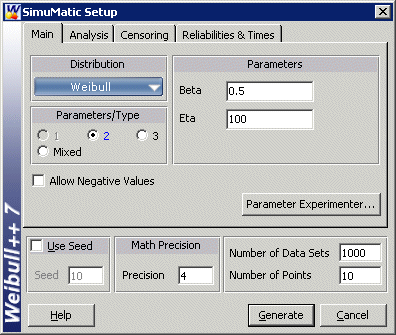
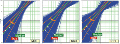
As an example, we will attempt to determine the best parameter estimation method for a sample of ten units following a Weibull distribution with [math]\displaystyle{ \beta }[/math] = 2 and [math]\displaystyle{ \eta }[/math] = 100 and with complete time-to-failure data for each unit (i.e., no censoring). Using SimuMatic, 10,000 data sets were generated (using Monte Carlo methods based on the Weibull distribution) and we estimated their parameters using RRX, RRY and MLE. The plotted results generated by SimuMatic are shown next.

The results clearly demonstrate that the median RRX estimate provides the least deviation from the truth for this sample size and data type. However, the MLE outputs are grouped more closely together, as evidenced by the confidence bounds. The same figures also show the simulation-based bounds, as well as the expected variation due to sampling error.

This experiment can be repeated in SimuMatic using multiple censoring schemes (including Type I and Type II right censoring as well as random censoring) with the included distributions. We can perform multiple experiments with this utility to evaluate our assumptions about the appropriate parameter estimation method to use for the data set.

Using Simulation to Design Reliability Tests

Good reliability specifications include requirements for reliability and an associated lower one-sided confidence interval. When designing a test, we must determine the sample size to test as well as the expected test duration. The next simple example illustrates the methods available in SimuMatic.

Example 8

Let us assume that a specific reliability specification states that at [math]\displaystyle{ T=10 }[/math] hr the reliability must be 99%, or [math]\displaystyle{ R(T=10)=99% }[/math] (unreliability = 1%), and at [math]\displaystyle{ T=20 }[/math] hr the reliability must be 90%, or [math]\displaystyle{ R(T=20)=90% }[/math] , at an 80% lower one-sided confidence level ( [math]\displaystyle{ L1S=80% }[/math] ).

One way to meet this specification is to design a test that will demonstrate either of these requirements at [math]\displaystyle{ L1S=80% }[/math] with the required parameters (for this example we will use the [math]\displaystyle{ R(T=10)=99% }[/math] @ [math]\displaystyle{ L1S=80% }[/math] requirement). With SimuMatic, we can specify the underlying distribution, distribution parameters (the Parameter Experimenter utility can be utilized), sample size on test, censoring scheme, required reliability and associated confidence level. From these inputs, SimuMatic will solve (via simulation) for the time demonstrated at the specified reliability and confidence level (i.e. [math]\displaystyle{ X }[/math] in the [math]\displaystyle{ R(T=X)=99% }[/math] @ [math]\displaystyle{ L1S=80% }[/math] formulation), as well as the expected test duration. If the demonstrated time is greater than the time requirement, this indicates that the test design would accomplish its required objective. Since there are multiple test designs that may accomplish the objective, multiple experiments should be performed until we arrive at an acceptable test design (i.e. number of units and test duration).

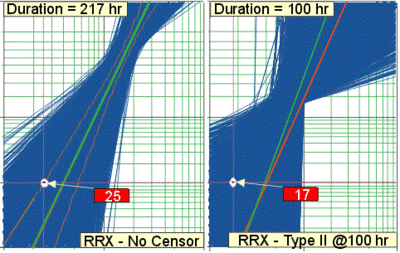
We start with a test design using a sample size of ten, with no censoring (i.e. all units to be tested to failure). We performed the analysis using RRX and 10,000 simulated data sets. The outcome is an expected test duration of 217 hr and a demonstrated time of 25 hr. This result is well above the stated requirement of 10 hr (note that in this case, the true value of T at a 50% CL, for R = 99%, is 40 hrs which gives us a ratio of 1.6 between true and demonstrated). Since this would demonstrate the requirement, we can then attempt to reduce the number of units or test time. Suppose that we need to bring the test time down to 100 hr (instead of the expected 217 hr). The test could then be designed using Type II censoring (i.e. any unit that has not failed by 100 hr is right censored) assuring completion by 100 hr. Again, we specify Type II censoring at 100 hr in SimuMatic, and we repeat the simulation with the same parameters as before. The simulation results in this case yield an expected test duration of 100 hr and a demonstrated time of 17 hr at the stated requirements. This result is also above our requirement The next figure graphically shows the results of this experiment. This process can then be repeated using different sample sizes and censoring schemes until we arrive at a desirable test plan.