Warranty Data Analysis: Difference between revisions
| Line 66: | Line 66: | ||
'''Quality In-Service Data''' | |||
[[File:ldachp12table3.png | [[File:ldachp12table3.png]] | ||
[[File:ldachp12table4.png|center]] | [[File:ldachp12table4.png|center]] | ||
Revision as of 18:29, 27 July 2011
Warranty Analysis
The Warranty Analysis Folio in Weibull++ provides three different data entry formats for warranty data. It also allows the user to automatically perform a life data analysis on this type of data, allows the prediction of future failures through the use of conditional probability analysis and provides methods for detecting outliers.
Warranty Data Entry Types
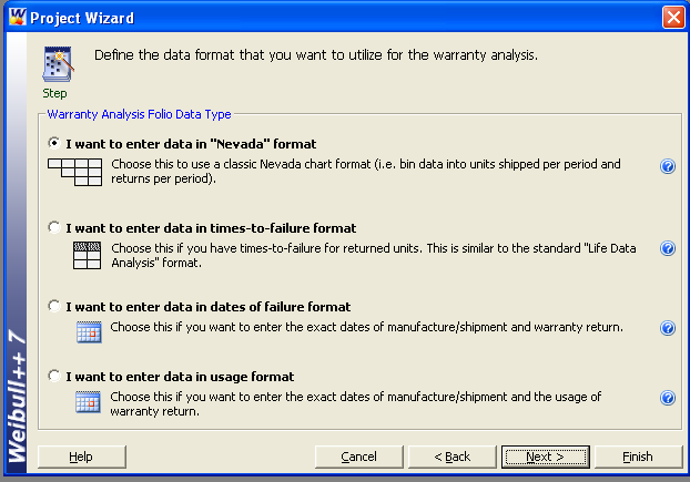
Weibull++ allows for data entry utilizing three common formats for storing sales and returns information. Specifically:
1) Nevada Chart Format
2) Time-to-Failure Format
3) Dates of Failure Format
4) Usage Format
These formats are explained in the next sections.
Nevada Chart Format
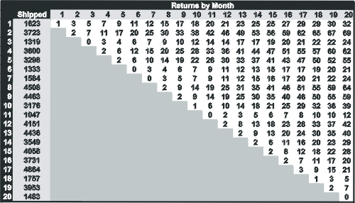
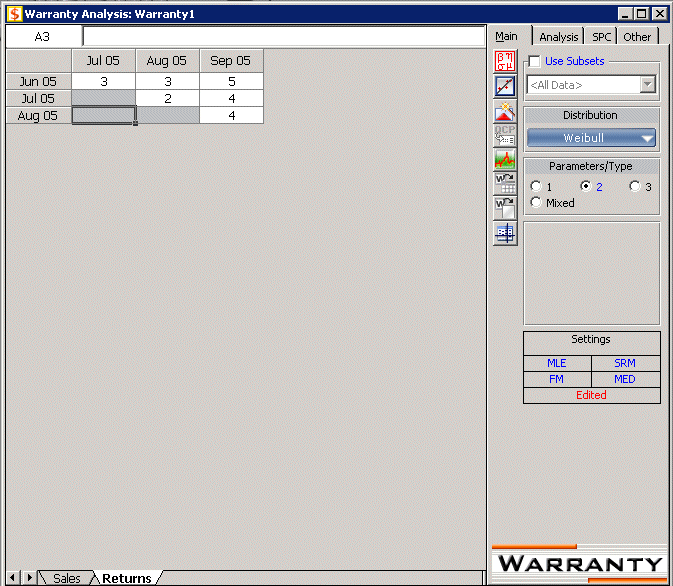
Field information frequently appears in terms of units produced and/or shipped in a certain time period, with the resulting returns for that production lot in the subsequent time periods. This information can be arranged in a diagonal chart, as displayed in the following figure.
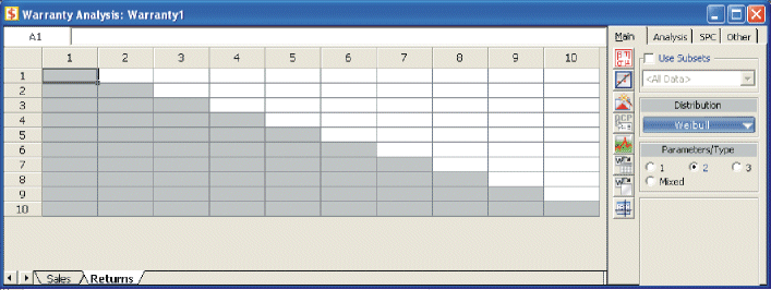
In Weibull++ this window is as shown next:
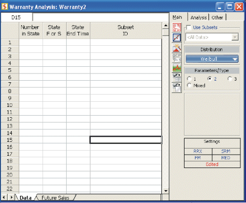
Time-to-Failure Format
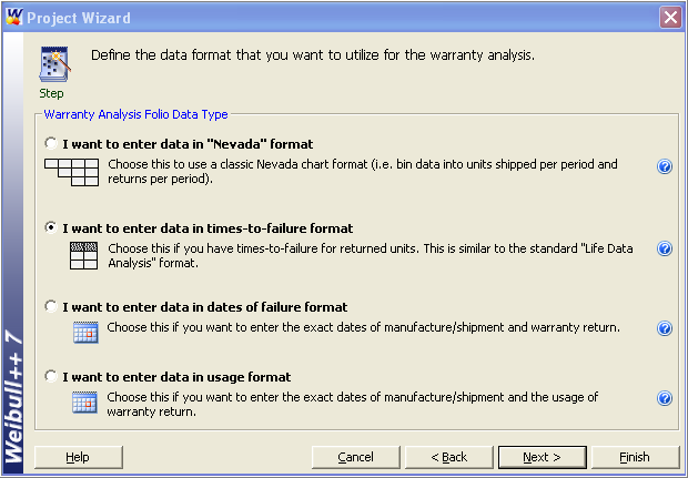
This format is similar to the Standard Folio data entry format (all number of units, failure times and suspension times are entered by the user), as discussed previously. The difference is that when the data is used within the context of warranty analysis, the automatic ability to generate forecasts is available to the user. In Weibull++ this window is as shown next:
Dates of Failure Format
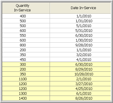
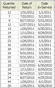
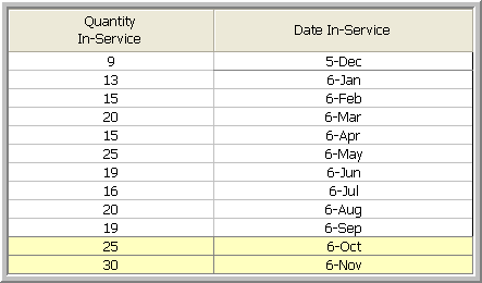
Another common way for reporting field information is to enter a date and quantity of sales or shipments, Quantity In-Service Data, and the date and quantity of returns, Quantity Returned Data, as illustrated in the following tables.
- Quality In-Service Data
- Quantity Returned Data
Note that in order to identify which lot the unit comes from, a failure is identified by a return date and the date of when it was put in service. The date that the unit went into service is then associated with the lot going into service during that time period. Lots can be used with the optional ID column which is covered in the sections that follow.
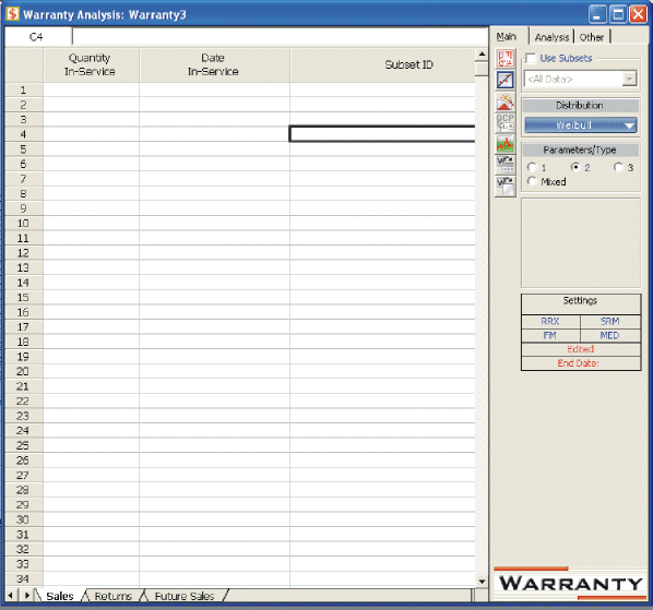
In Weibull++ this window is as shown next:
[math]\displaystyle{ }[/math]
Usage Format
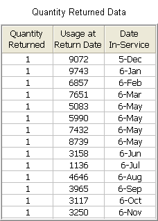
Often the driving factor for reliability is usage rather than time. For example, in the automotive industry, the failure behavior in the majority of the products is mileage-dependent rather than time-dependent. This format allows specifying Quantity In-Service Data, and the usage at return date and Quantity Return Data, as illustrated in the following tables.
Note that, like in the dates of failure format, in order to identify which lot the unit comes from, a failure is identified by the return number and the date of when it was put in service. The date that the returned unit went into service associates the returned unit with the lot it belonged to when it started operation. However, the return data is in terms of usage and not date of return. Therefore the usage of the units needs to be specified as a constant usage per unit time or as a distribution. This allows determining the expected usage of the surviving units (See Example 3).
Warranty Analysis (Nevada Format)
The Nevada Format allows the user to convert shipping and warranty return data into the standard reliability data form of failures and suspensions so that it can easily be analyzed with traditional life data analysis methods. For each time period in which a number of products are shipped, there will be a certain number of returns or failures in subsequent time periods, while the rest of the population that was shipped will continue to operate in the following time periods. For example, if 500 units are shipped in May, and 10 of those units are warranty returns in June, that is equivalent to 10 failures at a time of one month. The other 450 units will go on to operate and possibly fail in months that follow. At the end of the analysis period, all of the units that were shipped and have not failed in the time since shipment are considered to be suspensions. This process is repeated for each shipment and the results tabulated for each particular failure and suspension time prior to reliability analysis. This process may sound confusing, but it is actually just a matter of careful bookkeeping, and is illustrated with the example that follows.
Example 2
A company keeps track of its shipments and warranty returns on a month-by-month basis. The data format that the company uses is the Nevada format. Following is a table for shipments in June, July, and August, and the warranty returns through September:
- [math]\displaystyle{ \begin{matrix} {} & {} & RETURNS & {} & {} \\ {} & SHIP & \text{Jul}\text{. 2005} & \text{Aug}\text{. 2005} & \text{Sep}\text{. 2005} \\ \text{Jun}\text{. 2005} & \text{100} & \text{3} & \text{3} & \text{5} \\ \text{Jul}\text{. 2005} & \text{140} & \text{-} & \text{2} & \text{4} \\ \text{Aug}\text{. 2005} & \text{150} & \text{-} & \text{-} & \text{4} \\ \end{matrix} }[/math]
Convert this information to life data, and determine the parameters for a two-parameter Weibull distribution.
Solution to Example 2
We will examine the data month by month. In June 100 units were sold, and in July three of these units were returned. This gives three failures at one month for the June shipment, which we will denote as [math]\displaystyle{ {{F}_{JUN,1}}=3 }[/math] . Likewise, three failures occurred in August and five occurred in September for this shipment, or [math]\displaystyle{ {{F}_{JUN,2}}=3 }[/math] and [math]\displaystyle{ {{F}_{JUN,3}}=5. }[/math] Consequently, at the end of our three-month analysis period, there were a total of 11 failures for the 100 units shipped in June. This means that 89 units are presumably still operating, and can be considered suspensions at three months, or [math]\displaystyle{ {{S}_{JUN,3}}=89 }[/math] . For the shipment of 140 in July, two were returned the following month, or [math]\displaystyle{ {{F}_{JUL,1}}=2 }[/math] , and four more were returned the month after that, or [math]\displaystyle{ {{F}_{JUL,2}}=4. }[/math] After two months, there are 134 ( [math]\displaystyle{ 140-2-4=134 }[/math] ) units from the July shipment still operating, or [math]\displaystyle{ {{S}_{JUL,2}}=134 }[/math]. For the final shipment of 150 in August, four fail in September, or [math]\displaystyle{ {{F}_{AUG,1}}=4 }[/math], with the remaining 146 units being suspensions at one month, or [math]\displaystyle{ {{S}_{AUG,1}}=146 }[/math] .
It is now a simple matter to add up the number of failures for 1, 2, and 3 months, then add the suspensions to get our reliability data set:
- [math]\displaystyle{ \begin{matrix} \text{Failures at 1 month:} & {{F}_{1}}={{F}_{JUN,1}}+{{F}_{JUL,1}}+{{F}_{AUG,1}}=3+2+4=9 \\ \text{Suspensions at 1 month:} & {{S}_{1}}={{S}_{AUG,1}}=146 \\ \text{Failures at 2 months:} & {{F}_{2}}={{F}_{JUN,2}}+{{F}_{JUL,2}}=3+4=7 \\ \text{Suspensions at 2 months:} & {{S}_{2}}={{S}_{JUL,2}}=134 \\ \text{Failures at 3 months:} & {{F}_{3}}={{F}_{JUN,3}}=5 \\ \text{Suspensions at 3 months:} & {{S}_{JUN,3}}=89 \\ \end{matrix} }[/math]
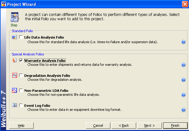
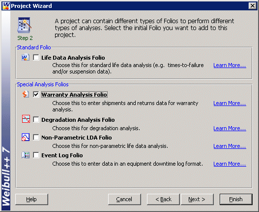
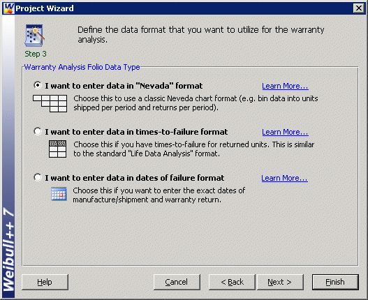
To perform this analysis using the Warranty Analysis tool in Weibull++, create a Warranty Analysis Folio and choose I want to enter data inNevada format in the Project Wizard.
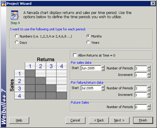
The next window allows you to specify the time units used. For this example select Months under I want to use the following unit type for each period and enter the Start month and Number of Periods and Increment number for the sales data and failure/return data as follows:
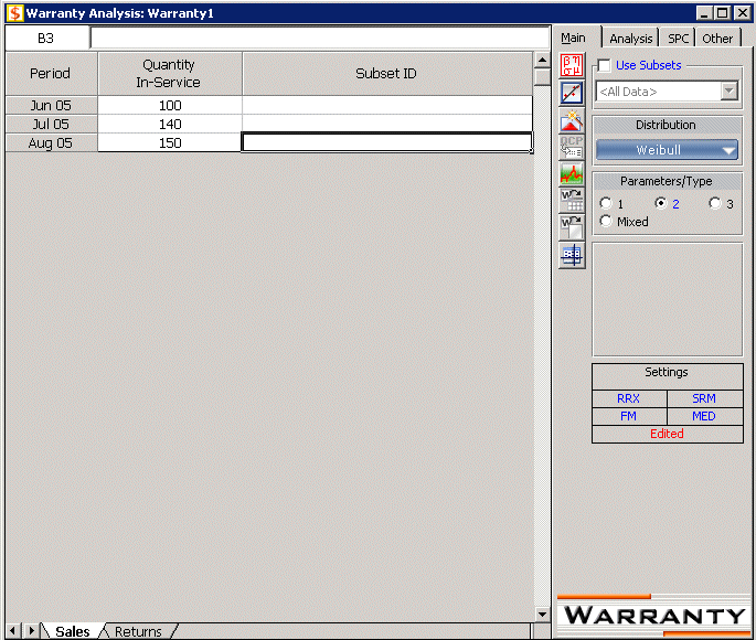
The sales data are entered as follows:
The return data are entered as follows:
The data can now be analyzed. Select two-parameter Weibull as the distribution type and MLE as the analysis method and click the Calculate button. The estimated parameters are [math]\displaystyle{ \widehat{\beta }=2.49 }[/math] and [math]\displaystyle{ \widehat{\eta }=6.70. }[/math]
Even though this step is not required for the analysis, the data can also be transferred to a Weibull++ data sheet for illustrative purposes or for ancillary analysis. This can be done by clicking the Transfer Life Data to New Folio button:
[math]\displaystyle{ }[/math]
or choosing this option under the Data menu.
The equivalent Times-to-failure folio is as follows:
Warranty Analysis (Usage Format)
Warranty data analysis relies on the estimation of a failure distribution based on data including the number of returns and the number of surviving units in the field and the age associated with those units. The Usage Format allows the user to convert shipping and warranty return data into the standard reliability data for of failures and suspensions when the return information is based on usage rather than return dates or periods.
Suppose that you have been collecting sales (units in service) and returns data. For the returns data, you can determine the number of failures and their usage (by reading the odometer value, for example). Determining the number of surviving units (suspensions) and their ages is a straightforward step. By taking the difference between the analysis date and the date when a unit was put in service, you can determine the age of the surviving units.
What is unknown, however, is the exact usage accumulated by each surviving unit. The key part of the usage-based warranty analysis is the determination of the usage of the surviving units based on their age. Therefore, the analyst needs to have an idea about the usage of the product. This can be obtained, for example, from customer surveys or by designing the products to collect usage data. For example, in automotive applications, engineers often use 12,000 miles/year as an average usage. Based on this average, the usage of an item that has been in the field for 6 months and has not yet failed would be 6,000 miles. So to obtain the usage of a suspension based on an average usage, one could take the time of each suspension and multiply it by this average usage. As you see, in this situation the analysis becomes straightforward. With the usage values and the quantities of the returned units, a failure distribution can be constructed and subsequent warranty analysis (such as warranty return forecasts described in 12.3.3) becomes possible.
Alternatively, and more realistically, instead of using an average usage, an actual distribution that reflects the variation in usage and customer behavior can be used. This distribution describes the usage of a unit over a certain time period (e.g. 1 year, 1 month, etc). This probabilistic model can be used to estimate the usage for all surviving components in service and the percentage of users running the product at different usage rates. In the automotive example, for instance, such a distribution can be used to calculate the percentage of customers that drive 0-200 miles/month, 200-400 miles/month, etc. We can take these percentages and multiply them by the number of suspensions to find the number of items that have been accumulating usage values in these ranges.
To proceed with applying a usage distribution, the usage distribution is divided into increments based on a specified interval width denoted as [math]\displaystyle{ Z }[/math] . The usage distribution, [math]\displaystyle{ Q }[/math] , is divided into intervals of [math]\displaystyle{ 0+Z }[/math] , [math]\displaystyle{ Z+Z }[/math] , [math]\displaystyle{ 2Z+Z }[/math] , etc., or [math]\displaystyle{ {{x}_{i}}={{x}_{i-1}}+Z }[/math] , as shown in the next figure.
The interval width should be selected such that it creates segments that are large enough to contain adequate numbers of suspensions within the intervals. The percentage of suspensions that belong to each usage interval is calculated as follows:
- [math]\displaystyle{ F({{x}_{i}})=Q({{x}_{i}})-Q({{x}_{i}}-1) }[/math]
Where:
- [math]\displaystyle{ Q() }[/math] is the usage distribution Cumulative Density Function, [math]\displaystyle{ cdf }[/math] .
- [math]\displaystyle{ x }[/math] represents the intervals used in apportioning the suspended population.
We also define a suspension group as a collection of suspensions that have the same age.
The above percentage of suspensions can be translated to numbers of suspensions within each interval, [math]\displaystyle{ {{x}_{i}} }[/math] . This is done by taking each group of suspensions and multiplying it by each [math]\displaystyle{ F({{x}_{i}}) }[/math] , or:
- [math]\displaystyle{ \begin{align} & {{N}_{1,j}}= & F({{x}_{1}})\times N{{S}_{j}} \\ & {{N}_{2,j}}= & F({{x}_{2}})\times N{{S}_{j}} \\ & & ... \\ & {{N}_{n,j}}= & F({{x}_{n}})\times N{{S}_{j}} \end{align} }[/math]
Where:
- [math]\displaystyle{ {{N}_{n,j}} }[/math] is the number of suspensions that belong to each interval.
- [math]\displaystyle{ N{{S}_{j}} }[/math] is the jth group of suspensions from the data set.
This is repeated for all the groups of suspensions.
The age of the suspensions is calculated by subtracting the Date In-Service ( [math]\displaystyle{ DIS }[/math] ), the date at which the unit started operation, from the calculation End Date ( [math]\displaystyle{ ED }[/math] ). This is the Time In-Service ( [math]\displaystyle{ TIS }[/math] ) value that describes the age of the surviving unit.
- [math]\displaystyle{ TIS=ED-DIS }[/math]
Note: [math]\displaystyle{ TIS }[/math] is in the same time units as the period in which the usage distribution is defined.
For each [math]\displaystyle{ {{N}_{k,j}} }[/math] , the usage is calculated as:
- [math]\displaystyle{ Uk,j=xi\times TISj }[/math]
After this step, the usage of each suspension group is estimated. The data can be combined with the failures and a failure distribution can be fitted.
Example 3
Suppose that an automotive manufacturer collects the warranty returns and sales data given in section 12.3.1.4 for a particular part in a given region. Convert this information to life data and fit a suitable distribution to it.
Solution to Example 3
To perform this analysis using the Warranty Analysis tool in Weibull++, create a Warranty Analysis Folio and choose I want to enter data in usage format in the Project Wizard. The sales data are entered as follows:
The return data (accumulated mileage at time of failure and the date the failed unit was put in-service ( [math]\displaystyle{ DIS }[/math] )) is shown in the next figure.
[math]\displaystyle{ }[/math]
The above figure also shows the calculation End Date ( [math]\displaystyle{ ED }[/math] ), which can be set on the Analysis page of the Control Panel. In this example, the warranty data were collected until 12/1/2006.
The user has the option to input either a constant value that describes an average of usage or a distribution with intervals to be considered in the analysis. In this example, the manufacturer has been documenting the mileage accumulation per year for this type of product across the customer base in comparable regions for many years. The yearly usage has been determined to follow a lognormal distribution with [math]\displaystyle{ {{\mu }_{T\prime }}=9.38 }[/math] , [math]\displaystyle{ {{\sigma }_{T\prime }}=0.085 }[/math] . Graphically, the distribution looks as follows.
[math]\displaystyle{ }[/math]
The usage distribution is specified on the Usage page of the Control Panel, as shown next.
[math]\displaystyle{ }[/math]
Note that the Interval Width was defined to be 1000 miles (as seen in the above figure). This interval facilitates the calculations of mileage usage for the suspensions in the data set.
In addition to 14 failures, the data set contains 212 suspensions spread according to the defined usage distribution. Note that due to rounding-off in the calculation, only 208 of these suspensions are ultimately allocated. This data set contains 12 groups of suspensions that have the same age. To illustrate the analysis procedure explained above, let us use one suspension group, the first group. The first group contains 9 units that went in service on a given date; 1 unit failed from that batch. Therefore, 8 suspensions have survived from December 2005 until the beginning of December 2006, a total of 12 months. The calculations are summarized as follows.
The two columns on the right constitute the calculated suspension data (number of suspensions and their usage) for the first group. The calculation in the above table is then repeated for each of the remaining 11 suspension groups in the data set. We then add the resulting data and the failure data and proceed with estimating a failure distribution model.
The data set that is used to perform the estimation of the failure distribution model can be extracted and displayed by selecting Transfer Life Data to New Folio from the Data menu. The failures and suspensions data set, as presented in the Standard Folio, is partially shown next. (Note that the Folio contains 66 rows.)
The entered sales and return data set, the usage distribution and the interval width in the Warranty Folio can be used to derive a failure distribution. The manufacturer assumes that the observed failures are typically modeled by a lognormal distribution. The parameters of the distribution are estimated (by clicking on the Calculate button) to be:
- [math]\displaystyle{ \begin{align} & {{\mu }_{T\prime }}= & 10.4747 \\ & {{\sigma }_{T\prime }}= & 1.1159 \end{align} }[/math]
The reliability plot (with mileage being the random variable driving reliability), along with the 90% confidence bounds on reliability, is shown next.
[math]\displaystyle{ }[/math]
Warranty Prediction
Once a life data analysis has been performed on warranty data, this information can be used to predict how many warranty returns there will be in subsequent time periods. This methodology uses the concept of conditional reliability (see Chapter 3) to calculate the probability of failure for the remaining units for each shipment time period. This conditional probability of failure is then multiplied by the number of units at risk from that particular shipment period that are still in the field (i.e. the suspensions) in order to predict the number of failures or warranty returns expected for this time period. The next example illustrates this.
Example 4
Using the data from Example 2, predict the number of warranty returns for October for each of the three shipment periods.
Solution to Example 4
We use the Weibull parameter estimates found in Example 2 to determine the conditional probability of failure for each shipment time period, and then multiply that probability with the number of units that are at risk for that period as follows. The equation for the conditional probability of failure is given by:
- [math]\displaystyle{ Q(t|T)=1-R(t|T)=1-\frac{R(T+t)}{R(T)} }[/math]
For the June shipment, there are 89 units that have successfully operated until the end of September ( [math]\displaystyle{ T=3 }[/math] [math]\displaystyle{ months) }[/math] . The probability of one of these units failing in the next month ( [math]\displaystyle{ t=1 }[/math] [math]\displaystyle{ month) }[/math] is then given by:
- [math]\displaystyle{ Q(1|3)=1-\frac{R(4)}{R(3)}=1-\frac{{{e}^{-{{\left( \tfrac{4}{6.70} \right)}^{2.49}}}}}{{{e}^{-{{\left( \tfrac{3}{6.70} \right)}^{2.49}}}}}=1-\frac{0.7582}{0.8735}=0.132 }[/math]
Once the probability of failure for an additional month of operation is determined, the expected number of failed units during the next month, from the June shipment, is the product of this probability and the number of units at risk ( [math]\displaystyle{ {{S}_{JUN,3}}=89) }[/math] or:
- [math]\displaystyle{ {{\widehat{F}}_{JUN,4}}=89\cdot 0.132=11.748\text{, or 12 units} }[/math]
This is then repeated for the July shipment, where there were 134 units operating at the end of September, with an exposure time of two months. The probability of failure in the next month is:
- [math]\displaystyle{ Q(1|2)=1-\frac{R(3)}{R(2)}=1-\frac{0.8735}{0.9519}=0.0824 }[/math]
This value is multiplied by [math]\displaystyle{ {{S}_{JUL,2}}=134 }[/math] to determine the number of failures, or:
- [math]\displaystyle{ {{\widehat{F}}_{JUL,3}}=134\cdot 0.0824=11.035\text{, or 11 units} }[/math]
For the August shipment, there were 146 units operating at the end of September, with an exposure time of one month. The probability of failure in the next month is:
- [math]\displaystyle{ Q(1|1)=1-\frac{R(2)}{R(1)}=1-\frac{0.9519}{0.9913}=0.0397 }[/math]
This value is multiplied by [math]\displaystyle{ {{S}_{AUG,1}}=146 }[/math] to determine the number of failures, or:
- [math]\displaystyle{ {{\widehat{F}}_{AUG,2}}=146\cdot 0.0397=5.796\text{, or 6 units} }[/math]
Thus, the total expected returns from all shipments for the next month is the sum of the above, or 29 units. This method can be easily repeated for different future sales periods, and utilizing projected shipments. If the user lists the number of units that are expected be sold or shipped during future periods, then these units are added to the number of units at risk whenever they are introduced into the field. The warranty analysis tool in Weibull++ performs this type of analysis for you.
Note that Weibull++ can perform this step automatically by using the `Generate Forecast' functionality.
Analysis of Non-Homogeneous Warranty Data
In the previous sections and examples it is important to note that the underlying assumption was that the population was homogeneous. In other words, all sold and returned units were exactly the same, i.e. the same population with no design changes and/or modifications. In many situations, as the product matures, design changes are made to enhance and/or improve the reliability of the product. Obviously, an improved product will exhibit different failure characteristics than its predecessor. To analyze such cases, where the population is non-homogeneous, one needs to extract each homogenous group, fit a life model to each group and then project the expected returns for each group based on the number of units at risk for each specific group.
Using IDs in Weibull++
Weibull++ 7 uses the optional IDs column to differentiate between product versions or different designs (lots). Based on this entry, the data are then automatically separated and the parameters for each lot computed. Based on the computed parameters, failure projections can then be obtained. Note that it is important to realize that the same limitations as discussed previously, with regards to the number of failures that are needed, are also applicable here. In other words, distributions can be automatically fitted to lots that have return (failure) data, whereas if no returns have been experienced yet (either because the units are going to be introduced in the future or because no failures happened yet), the user will be asked to specify the parameters, since they can not be computed. Consequently, subsequent estimation/predictions related to these lots would be based on the user specified parameters. Following is an example that illustrates the use of IDs.
Example 5
A company keeps track of its production and returns. The company uses the `Dates of Failure' format to record the data. For the product in question, three versions (A, B and C) have been produced and put in service.
The in-service data is as follows (using the US date format of Month/Day/Year):
- [math]\displaystyle{ \begin{matrix} Quantity In-Service & Date of In-Service & ID \\ \text{400} & \text{1/1/2005} & \text{Model A} \\ \text{500} & \text{1/31/2005} & \text{Model A} \\ \text{500} & \text{5/1/2005} & \text{Model A} \\ \text{600} & \text{5/31/2005} & \text{Model A} \\ \text{550} & \text{6/30/2005} & \text{Model A} \\ \text{600} & \text{7/30/2005} & \text{Model A} \\ \text{800} & \text{9/28/2005} & \text{Model A} \\ \text{200} & \text{1/1/2005} & \text{Model B} \\ \text{350} & \text{3/2/2005} & \text{Model B} \\ \text{450} & \text{4/1/2005} & \text{Model B} \\ \text{300} & \text{6/30/2005} & \text{Model B} \\ \text{200} & \text{8/29/2005} & \text{Model B} \\ \text{350} & \text{10/28/2005} & \text{Model B} \\ \text{1100} & \text{2/1/2005} & \text{Model C} \\ \text{1200} & \text{3/27/2005} & \text{Model C} \\ \text{1200} & \text{4/25/2005} & \text{Model C} \\ \text{1300} & \text{6/1/2005} & \text{Model C} \\ \text{1400} & \text{8/26/2005} & \text{Model C} \\ \end{matrix} }[/math]
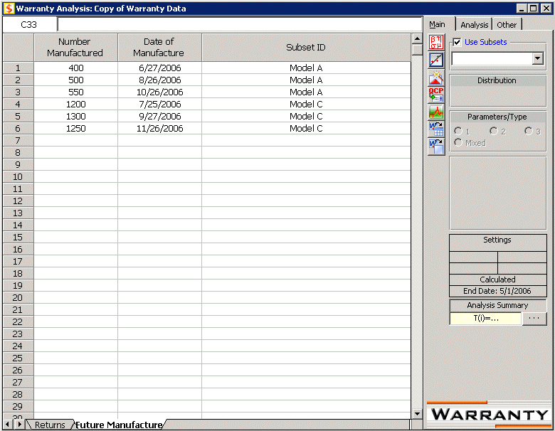
Furthermore, the following sales are forecast:
- [math]\displaystyle{ \begin{matrix} Number & Date & ID \\ \text{400} & \text{6/27/2006} & \text{Model A} \\ \text{500} & \text{8/26/2006} & \text{Model A} \\ \text{550} & \text{10/26/2006} & \text{Model A} \\ \text{1200} & \text{7/25/2006} & \text{Model C} \\ \text{1300} & \text{9/27/2006} & \text{Model C} \\ \text{1250} & \text{11/26/2006} & \text{Model C} \\ \end{matrix} }[/math]
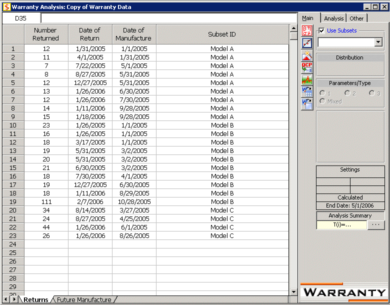
The return data are as follows. Note that in order to identify which lot each unit comes from and be able to compute its time-in-service, each return (failure) includes a return date, the date of when it was put in service and the Model (ID).
Assuming that the above information is as of 5/1/2006, analyze the data using the lognormal as the assumed distribution and MLE as the analysis method, for all models (Model A, Model B, Model C), and provide a return forecast for the next ten months.
Solution to Example 5
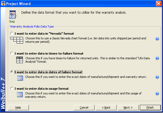
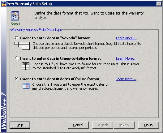
Create a warranty folio by clicking on Project and choosing Add Specialized Folio and then selecting Add Warranty. In the New Warranty Folio Setup window, choose I want to enter data in dates of failure format.
The return data are entered as follows:
The sales data are entered as follows (note that the Use Subsets check box should be checked):
Under the Analysis tab, set the Calculations End Date to (5/1/2006) as shown next:
The calculated parameters, assuming a lognormal distribution and using MLE as the analysis method, are:
- [math]\displaystyle{ \begin{matrix} Model A & Model B & Model C \\ \begin{matrix} {{{\hat{\mu }}}^{\prime }}= & \text{11}\text{.28} \\ {{{\hat{\sigma }}}_{T}}= & \text{2}\text{.83} \\ \end{matrix} & \begin{matrix} {{{\hat{\mu }}}^{\prime }}= & \text{8}\text{.11} \\ {{{\hat{\sigma }}}_{T}}= & \text{2}\text{.30} \\ \end{matrix} & \begin{matrix} {{{\hat{\mu }}}^{\prime }}= & \text{9}\text{.79} \\ {{{\hat{\sigma }}}_{T}}= & \text{1}\text{.92} \\ \end{matrix} \\ \end{matrix} }[/math]
Note that in this example, the same distribution type and analysis method were assumed for each of the product models. If desired, different distribution types, analysis methods, confidence bounds methods, etc., can be assumed for each IDs.
To obtain the expected failures for the next 10 months, click the Generate Forecast button.
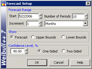
and enter the Start date of 5/2/2006, the Number of Periods as 10, and the Increment number (1) in Months (selected from the drop-down box), as shown next:
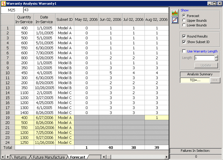
The forecast results are then displayed in a new sheet called Forecast. Part of the forecast table is shown next.
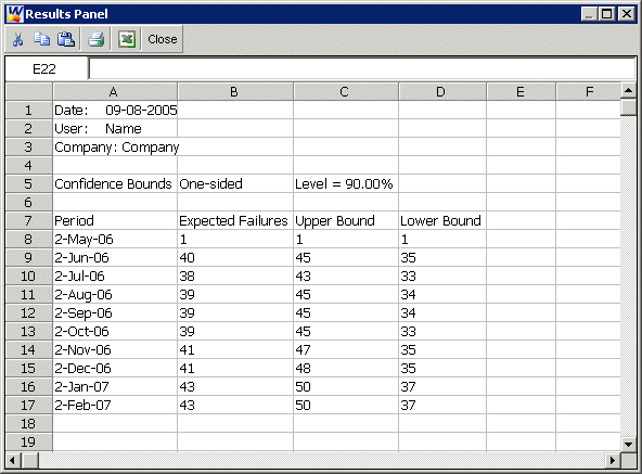
A summary of the analysis can also be obtained by clicking on the Show Analysis Summary (...). The summary of the forecasted returns is as follows:
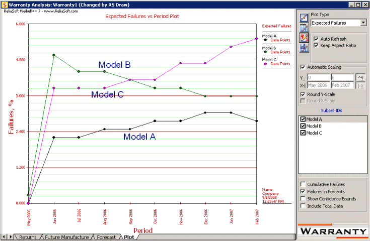
The results can also be seen graphically in the following plot. This is a plot of the expected failures (in percent).
Monitoring Warranty Returns Using Statistical Process Control (SPC)
By monitoring and analyzing warranty return data, the user now has the ability to detect specific return periods and/or batches of sales or shipments that may deviate (differ) from the assumed model. This provides the analyst (and the organization) the advantage of early notification of possible deviations in manufacturing, use conditions and/or any other factor that may adversely affect the reliability of the fielded product.
Obviously, the motivation for performing such analysis is to allow for faster intervention to avoid increased costs due to increased warranty returns or more serious repercussions. Additionally, this analysis can also be used to uncover different sub-populations that may exist within this population.
Analysis Method
For each sales period [math]\displaystyle{ i }[/math] and return period [math]\displaystyle{ j }[/math] , the prediction error can be calculated as follows:
- [math]\displaystyle{ {{e}_{i,j}}={{\hat{F}}_{i,j}}-{{F}_{i,j}} }[/math]
where [math]\displaystyle{ {{\hat{F}}_{i,j}} }[/math] is the estimated number of failures based on the estimated distribution parameters for the sales period [math]\displaystyle{ i }[/math] and the return period [math]\displaystyle{ j }[/math] , which is calculated using Eqn.(Conditional), and [math]\displaystyle{ {{F}_{i,j}} }[/math] is the actual number of failure for the sales period [math]\displaystyle{ i }[/math] and the return period [math]\displaystyle{ j }[/math] .
Since we are assuming that the model is accurate, [math]\displaystyle{ {{e}_{i,j}} }[/math] should follow a normal distribution with mean value of zero and a standard deviation [math]\displaystyle{ s }[/math] , where:
- [math]\displaystyle{ {{\bar{e}}_{i,j}}=\frac{\underset{i}{\mathop{\sum }}\,\underset{j}{\mathop{\sum }}\,{{e}_{i,j}}}{n}=0 }[/math]
and [math]\displaystyle{ n }[/math] is the total number of return data (total number of residuals).
The estimated standard deviation of the prediction errors can then be calculated by:
- [math]\displaystyle{ s=\sqrt{\frac{1}{n-1}\underset{i}{\mathop \sum }\,\underset{j}{\mathop \sum }\,e_{i,j}^{2}} }[/math]
and [math]\displaystyle{ {{e}_{i,j}} }[/math] can be normalized as follows:
- [math]\displaystyle{ {{z}_{i,j}}=\frac{{{e}_{i,j}}}{s} }[/math]
where [math]\displaystyle{ {{z}_{i,j}} }[/math] is the standardized error. [math]\displaystyle{ {{z}_{i,j}} }[/math] follows a normal distribution with [math]\displaystyle{ \mu =0 }[/math] and [math]\displaystyle{ \sigma =1 }[/math] .
It is known that the square of a random variable with standard normal distribution follows the [math]\displaystyle{ {{\chi }^{2}} }[/math] (Chi Square) distribution with 1 degree of freedom and that the sum of the squares of [math]\displaystyle{ m }[/math] random variables with standard normal distribution follows the [math]\displaystyle{ {{\chi }^{2}} }[/math] distribution with [math]\displaystyle{ m }[/math] degrees of freedom [math]\displaystyle{ . }[/math] This then can be used to help detect the abnormal returns for a given sales period, return period or just a specific cell (combination of a return and a sales period).
• For a cell, abnormality is detected if [math]\displaystyle{ z_{i,j}^{2}=\chi _{1}^{2}\ge \chi _{1,\alpha }^{2}. }[/math]
• For an entire sales period [math]\displaystyle{ i }[/math] , abnormality is detected if [math]\displaystyle{ \underset{j}{\mathop{\sum }}\,z_{i,j}^{2}=\chi _{J}^{2}\ge \chi _{\alpha ,J}^{2}, }[/math] where [math]\displaystyle{ J }[/math] is the total number of return period for a sales period [math]\displaystyle{ i }[/math] .
• For an entire return period [math]\displaystyle{ j }[/math] , abnormality is detected if [math]\displaystyle{ \underset{i}{\mathop{\sum }}\,z_{i,j}^{2}=\chi _{I}^{2}\ge \chi _{\alpha ,I}^{2}, }[/math] where [math]\displaystyle{ I }[/math] is the total number of sales period for a return period [math]\displaystyle{ j }[/math] . Here [math]\displaystyle{ \alpha }[/math] is the criticality value of the [math]\displaystyle{ {{\chi }^{2}} }[/math] distribution, which can be set at critical value or caution value. It describes the level of sensitivity to outliers (returns that deviate significantly from the predictions based on the fitted model). Increasing the value of [math]\displaystyle{ \alpha }[/math] increases the power of detection, but this could lead to more false alarms.
Example 6
Using the same data from Example 2, the expected returns for each sales period can be obtained using conditional reliability concepts, as given in Eqn.(Conditional). For example, for the third return month of the first sales period, the expected return number is given by:
- [math]\displaystyle{ {{\hat{F}}_{Jun,3}}=(100-6)\cdot \left( 1-\frac{R(3)}{R(2)} \right)=94\cdot 0.08239=7.7447 }[/math]
The actual returns in this period were five, thus the prediction error for this period is:
- [math]\displaystyle{ {{e}_{Jun,3}}={{\hat{F}}_{Jun,3}}-{{F}_{Jun,3}}=7.7447-5=2.7447. }[/math]
This can then be repeated for each cell, yielding the following table for [math]\displaystyle{ {{e}_{i,j}} }[/math] :
- [math]\displaystyle{ \begin{matrix} {} & {} & RETURNS & {} & {} \\ {} & SHIP & \text{Jul}\text{. 2005} & \text{Aug}\text{. 2005} & \text{Sep}\text{. 2005} \\ \text{Jun}\text{. 2005} & \text{100} & \text{-2}\text{.1297} & \text{0}\text{.8462} & \text{2}\text{.7447} \\ \text{Jul}\text{. 2005} & \text{140} & \text{-} & \text{-0}\text{.7816} & \text{1}\text{.4719} \\ \text{Aug}\text{. 2005} & \text{150} & \text{-} & \text{-} & \text{-2}\text{.6946} \\ \end{matrix} }[/math]
Now, for this example, [math]\displaystyle{ n=6 }[/math] , [math]\displaystyle{ {{\bar{e}}_{i,j}}=-0.5432 }[/math] and [math]\displaystyle{ s=1.6890. }[/math]
Thus the .. values are:
- [math]\displaystyle{ \begin{matrix} {} & {} & RETURNS & {} & {} \\ {} & SHIP & \text{Jul}\text{. 2005} & \text{Aug}\text{. 2005} & \text{Sep}\text{. 2005} \\ \text{Jun}\text{. 2005} & \text{100} & \text{-0}\text{.9968} & \text{0}\text{.3960} & \text{1}\text{.2846} \\ \text{Jul}\text{. 2005} & \text{140} & \text{-} & \text{-0}\text{.3658} & \text{0}\text{.6889} \\ \text{Aug}\text{. 2005} & \text{150} & \text{-} & \text{-} & \text{-1}\text{.2612} \\ \end{matrix} }[/math]
The [math]\displaystyle{ z_{i,j}^{2} }[/math] .. values, for each cell, are given in the following table.
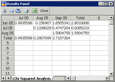
- [math]\displaystyle{ \begin{matrix} {} & {} & RETURNS & {} & {} & {} \\ {} & SHIP & \text{Jul}\text{. 2005} & \text{Aug}\text{. 2005} & \text{Sep}\text{. 2005} & \text{Sum} \\ \text{Jun}\text{. 2005} & \text{100} & \text{0}\text{.9936} & \text{0}\text{.1569} & \text{1}\text{.6505} & 2.8010 \\ \text{Jul}\text{. 2005} & \text{140} & \text{-} & \text{0}\text{.1338} & \text{0}\text{.4747} & 0.6085 \\ \text{Aug}\text{. 2005} & \text{150} & \text{-} & \text{-} & \text{1}\text{.5905} & 1.5905 \\ \text{Sum} & {} & 0.9936 & 0.2907 & 3.7157 & {} \\ \end{matrix} }[/math]
If the critical value is set at [math]\displaystyle{ \alpha = }[/math] 0.01 and the caution value is set at [math]\displaystyle{ \alpha = }[/math] 0.1, then the critical and caution [math]\displaystyle{ {{\chi }^{2}} }[/math] values will be:
- [math]\displaystyle{ \begin{matrix} {} & Degree of Freedom & {} & {} \\ {} & \text{1} & \text{2} & \text{3} \\ {{\chi }^{2}} & & & \\ & & & \\ \end{matrix} }[/math]
If we consider sales periods as the basis foroutlier detection, then after comparing the above table to the sum of [math]\displaystyle{ z_{i,j}^{2} }[/math] [math]\displaystyle{ (\chi _{1}^{2}) }[/math] values for each sales period, we find that all the sales values do not exceed the critical and caution limits.
For example, the total [math]\displaystyle{ {{\chi }^{2}} }[/math] value of the sale month of July is 0.6085. Its degrees of freedom is 2, so the corresponding caution and critical values are 4.6052 and 9.2103 respectively. Both values are larger than 0.6085, so the return numbers of the July sales period do not deviate (based on the chosen significance) from the model's predictions. If we consider returns periods as the basis foroutliers detection, then after comparing the above table to the sum of [math]\displaystyle{ z_{i,j}^{2} }[/math] [math]\displaystyle{ (\chi _{1}^{2}) }[/math] values for each return period, we find that all the return values do not exceed the critical and caution limits. For example, the total [math]\displaystyle{ {{\chi }^{2}} }[/math] value of the sale month of August is 3.7157. Its degree of freedom is 3, so the corresponding caution and critical values are 6.2514 and 11.3449 respectively. Both values are larger than 3.7157, so the return numbers for the June return period do not deviate from the model's predictions.
The above analysis can be automatically performed in Weibull++ by entering the alpha values under the SPC tab and selecting what type of color code to use, under Color Code Returns Sheet.
The Chi Squared values ( [math]\displaystyle{ z_{i,j}^{2} }[/math]
- [math]\displaystyle{ \begin{matrix} Period & Quantity In-Service \\ \text{Sep 05} & \text{1150} \\ \text{Oct 05} & \text{1100} \\ \text{Nov 05} & \text{1200} \\ \text{Dec 05} & \text{1155} \\ \text{Jan 06} & \text{1255} \\ \text{Feb 06} & \text{1150} \\ \text{Mar 06} & \text{1105} \\ \text{Apr 06} & \text{1110} \\ \end{matrix} }[/math]
or [math]\displaystyle{ \chi _{1}^{2} }[/math] values) can be seen in the next figure (obtained by clicking the (...) button under the SPC tab).
Weibull++ automatically color codes SPC results for easy visualization in the returns data sheet. By default the green color means that the return number is normal; the yellow color indicates that the return number is larger than the caution threshold but smaller than the critical value; the red color means that the return is abnormal, meaning that the return number is either too big or too small compared to the predicted value.
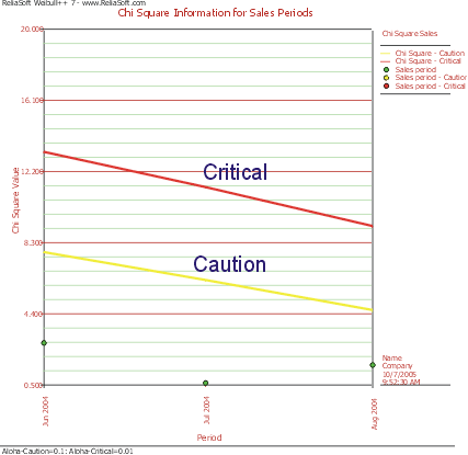
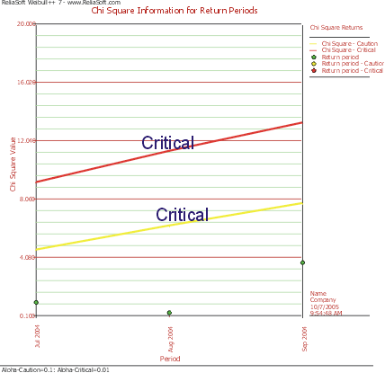
In this example, all the cells are coded in green for both analyses, i.e. By Sales Periods or By Return Periods, indicating that all returns fall within the caution and critical limits (i.e. nothing abnormal). Another way to visualize this is by using a Chi-Square plot as shown in the next two figures.
The Chi-Square plot for sales is:
The Chi-square plot for returns is:
Example 7
The SPC (warranty monitoring) methodology explained in this section can also be used to detect different subpopulations. The different subpopulations can reflect different use conditions, different material, etc. In this methodology, one can use different IDs to differentiate between subpopulations, and obtain models that are distinct to each subpopulation. The following example illustrates this concept. A manufacturer collected the following sales and return data.
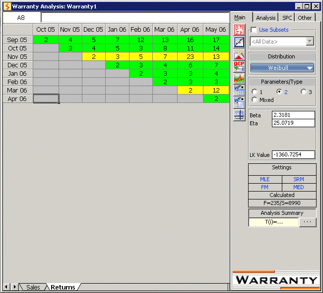
- [math]\displaystyle{ \begin{matrix} {} & Oct 05 & Nov 05 & Dec 05 & Jan 06 & Feb 06 & Mar 06 & Apr 06 & May 06 \\ Sep 05 & \text{2} & \text{4} & \text{5} & \text{7} & \text{12} & \text{13} & \text{16} & \text{17} \\ Oct 05 & \text{-} & \text{3} & \text{4} & \text{5} & \text{3} & \text{8} & \text{11} & \text{14} \\ Nov 05 & \text{-} & \text{-} & \text{2} & \text{3} & \text{5} & \text{7} & \text{23} & \text{13} \\ Dec 05 & \text{-} & \text{-} & \text{-} & \text{2} & \text{3} & \text{4} & \text{6} & \text{7} \\ Jan 06 & \text{-} & \text{-} & \text{-} & \text{-} & \text{2} & \text{3} & \text{3} & \text{4} \\ Feb 06 & \text{-} & \text{-} & \text{-} & \text{-} & \text{-} & \text{2} & \text{3} & \text{3} \\ Mar 06 & \text{-} & \text{-} & \text{-} & \text{-} & \text{-} & \text{-} & \text{2} & \text{12} \\ Apr 06 & \text{-} & \text{-} & \text{-} & \text{-} & \text{-} & \text{-} & \text{-} & \text{2} \\ \end{matrix} }[/math]
The data were analyzed using the two-parameter Weibull distribution and the MLE analysis method. The parameters are estimated to be:
- [math]\displaystyle{ \begin{align} & \beta = & 2.31 \\ & \eta = & 25.07 \end{align} }[/math]
The SPC's [math]\displaystyle{ \alpha }[/math] value are set at 0.01 for the Critical Value and 0.1 for the Caution Value. When analyzed and color coded in Weibull++ the following window is obtained:
Here the Nov. 05 and Mar 06 sales periods are colored in yellow indicating that they are `outlier' sales periods, while the rest are green. One suspected reason for the variation may be the material used in production in this period. Further analysis confirmed that for these periods the material was acquired from a different supplier. This then implies that the units are not homogenous, and that there are different subpopulations present in the field populations.
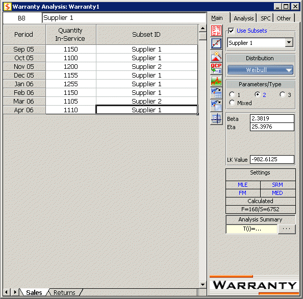
Based on this, the data is re-analyzed after categorizing the different shipments (using the ID column) based on their material supplier. The data as entered are shown next.
The new models that describe the data are (assuming a two-parameter Weibull distribution and using MLE as the analysis method for both sub-populations):
- [math]\displaystyle{ \begin{matrix} Supplier 1 & Supplier 2 \\ \begin{matrix} \beta =2.38 \\ \eta =25.39 \\ \end{matrix} & \begin{matrix} \beta =2.32 \\ \eta =21.28 \\ \end{matrix} \\ \end{matrix} }[/math]
This analysis helped in uncovering different subpopulations as well as allowing us to compute different distributions for each subpopulation. Note that if the analysis were performed on the failure and suspension times in a regular Standard Folio, using the mixed Weibull distribution, one would not be able to detect which units fall into which subpopulation.

