Logistic: Difference between revisions
| Line 31: | Line 31: | ||
<br> | <br> | ||
<br> | <br> | ||
<br> | <br> | ||
{|style= align="center" border="1" | {|style= align="center" border="1" | ||
|+Table 8.1 - Development time versus observed reliability data and predicted reliabilities | |||
!Time, months | !Time, months | ||
!Raw Data Reliability (%) | !Raw Data Reliability (%) | ||
| Line 81: | Line 81: | ||
<br> | <br> | ||
[[File:rga8.1.png|center]] | [[File:rga8.1.png|center]] | ||
< | <center>Figure 8.1: Estimated Standard Gompertz parameters for Example 1.</center> | ||
<br> | <br> | ||
<br> | <br> | ||
<br> | <br> | ||
[[File:rga8.2.png|center]] | [[File:rga8.2.png|center]] | ||
< | <center>Figure 8.2: Gompertz Reliability vs. Time plot.</center> | ||
<br> | <br> | ||
<br> | <br> | ||
| Line 136: | Line 134: | ||
<br> | <br> | ||
[[File:rga8.3.png|center]] | [[File:rga8.3.png|center]] | ||
< | <center>Figure 8.3: Logistic Reliability vs. Time plot.</center> | ||
| Line 147: | Line 144: | ||
<br> | <br> | ||
<br> | <br> | ||
{|style= align="center" border="1" | {|style= align="center" border="1" | ||
|+Table 8.2 - Sequential success/failure data with observed reliability values | |||
!Time | !Time | ||
!Result | !Result | ||
| Line 234: | Line 231: | ||
<br> | <br> | ||
<br> | <br> | ||
{|style= align="center" border="1" | {|style= align="center" border="1" | ||
|+Table 8.3 - Grouped per configuration data | |||
!Number of Units | !Number of Units | ||
!Number of Failures | !Number of Failures | ||
| Line 312: | Line 309: | ||
<math></math> | <math></math> | ||
[[File:rga8.4.png|center]] | [[File:rga8.4.png|center]] | ||
< | <center>Figure 8.4: Logistic Reliability vs. Time plot.</center> | ||
<br> | <br> | ||
<br> | <br> | ||
| Line 320: | Line 316: | ||
<br> | <br> | ||
[[File:rga8.5.png|center]] | [[File:rga8.5.png|center]] | ||
< | <center>Figure 8.5: Logistic Reliability vs. Time plot displaying the intervals.</center> | ||
<br> | <br> | ||
<br> | <br> | ||
| Line 422: | Line 417: | ||
<math></math> | <math></math> | ||
[[File:rga8.6.png|center]] | [[File:rga8.6.png|center]] | ||
< | <center>Figure 8.6: Logistic Reliability vs. Time plot with 2-sided 90% confidence bounds.</center> | ||
==General Examples== | ==General Examples== | ||
| Line 440: | Line 434: | ||
<br> | <br> | ||
<br> | <br> | ||
{|style= align="center" border="1" | {|style= align="center" border="1" | ||
|+Table 8.4 - Reliability data | |||
!Month | !Month | ||
!Observed Reliability(%) | !Observed Reliability(%) | ||
| Line 473: | Line 467: | ||
<br> | <br> | ||
[[File:rga8.7.png|center]] | [[File:rga8.7.png|center]] | ||
< | <center>Figure 8.7: Entered data and the estimated Logistic parameters.</center> | ||
<br> | <br> | ||
<br> | <br> | ||
<br> | <br> | ||
[[File:rga8.8.png|center]] | [[File:rga8.8.png|center]] | ||
< | <center>Figure 8.8: Reliability vs. Time plot.</center> | ||
<br> | <br> | ||
<br> | <br> | ||
<br> | <br> | ||
[[File:rga8.9.png|center]] | [[File:rga8.9.png|center]] | ||
< | <center>Figure 8.9: When the reliability goal of 99% will be achieved.</center> | ||
<br> | <br> | ||
<br> | <br> | ||
<br> | <br> | ||
[[File:rga8.10.png|center]] | [[File:rga8.10.png|center]] | ||
<center>Figure 8.10: The reliability at the end of the following January (month=20)</center> | |||
<br> | <br> | ||
====Solution to Example 5==== | ====Solution to Example 5==== | ||
| Line 524: | Line 513: | ||
<br> | <br> | ||
<br> | <br> | ||
{|style= align="center" border="1" | {|style= align="center" border="1" | ||
|+Table 8.5 - Sequential success/failure data | |||
!Launch Number | !Launch Number | ||
!Result | !Result | ||
| Line 584: | Line 573: | ||
<math></math> | <math></math> | ||
[[File:rga8.11.png|center]] | [[File:rga8.11.png|center]] | ||
< | <center>Figure 8.11: Entered data and the estimated logistic parameters.</center> | ||
<br> | <br> | ||
<br> | <br> | ||
<br> | <br> | ||
[[File:rga8.12.png|center]] | [[File:rga8.12.png|center]] | ||
< | <center>Figure 8.12: Reliability vs. Time plot.</center> | ||
<br> | <br> | ||
<br> | <br> | ||
<br> | <br> | ||
[[File:rga8.13.png|center]] | [[File:rga8.13.png|center]] | ||
< | <center>Figure 8.13: When the reliability goal of 99.5% with a 90% confidence level will be achieved.</center> | ||
<br> | <br> | ||
<br> | <br> | ||
<br> | <br> | ||
[[File:rga8.14.png|center]] | [[File:rga8.14.png|center]] | ||
< | <center>Figure 8.14: The reliability at the end of the 35th launch.</center> | ||
<br> | <br> | ||
<br> | <br> | ||
| Line 623: | Line 608: | ||
<br> | <br> | ||
<br> | <br> | ||
{|style= align="center" border="1" | {|style= align="center" border="1" | ||
|+Table 8.6 - Sequential success/failure data with modes | |||
!Launch Number | !Launch Number | ||
!Result | !Result | ||
| Line 683: | Line 668: | ||
<math></math> | <math></math> | ||
[[File:rga8.15.png|center]] | [[File:rga8.15.png|center]] | ||
< | <center>Figure 8.15: Entered data and the estimated Logistic parameters.</center> | ||
<br> | <br> | ||
<br> | <br> | ||
| Line 695: | Line 679: | ||
<br> | <br> | ||
[[File:rga8.17.png|center]] | [[File:rga8.17.png|center]] | ||
< | <center>Figure 8.17: Calculate when the reliability goal of 99.5% will be achieved.</center> | ||
<br> | <br> | ||
<br> | <br> | ||
<br> | <br> | ||
[[File:rga8.18.png|center]] | [[File:rga8.18.png|center]] | ||
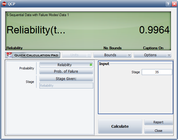
< | <center>Figure 8.18: Calculate the reliability at the end of the 35th launch.</center> | ||
Revision as of 00:16, 5 August 2011
Logistic
The Logistic reliability growth model has an S-shaped curve and is given by [3]:
where [math]\displaystyle{ b }[/math] and [math]\displaystyle{ k }[/math] are parameters. Similar to the analysis given for the Gompertz curve (Chapter 7), the following may be concluded:
1) The point of inflection is given by:
- [math]\displaystyle{ {{T}_{i}}=\frac{\ln (b)}{k} }[/math]
2) When [math]\displaystyle{ b\gt 1 }[/math] then [math]\displaystyle{ {{T}_{i}}\gt 0 }[/math] and an S-shaped curve will be generated. However, w[math]\displaystyle{ % }[/math]hen [math]\displaystyle{ 0\lt b\le 1 }[/math] then [math]\displaystyle{ {{T}_{i}}\le 0 }[/math] and the Logistic reliability growth model will not be described by an S-shaped curve.
3) The value of [math]\displaystyle{ R }[/math] is equal to 0.5 at the inflection point.
Parameter Estimation
Example 1
Using the reliability growth data given in Table 8.1, do the following:
1) Find a Gompertz curve that represents the data and plot it with the raw data.
2) Find a Logistic reliability growth curve that represents the data and plot it with the raw data.
| Time, months | Raw Data Reliability (%) | Gompertz Reliability (%) | Logistic Reliablity (%) |
|---|---|---|---|
| 0 | 31.00 | 24.85 | 22.73 |
| 1 | 35.50 | 38.48 | 38.14 |
| 2 | 49.30 | 51.95 | 56.37 |
| 3 | 70.10 | 63.82 | 73.02 |
| 4 | 83.00 | 73.49 | 85.01 |
| 5 | 92.20 | 80.95 | 92.24 |
| 6 | 96.40 | 86.51 | 96.14 |
| 7 | 98.60 | 90.54 | 98.12 |
| 8 | 99.00 | 93.41 | 99.09 |
Solution
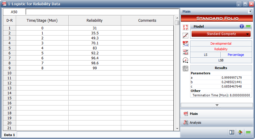
1) Figure Logistic1 shows the entered data and the estimated parameters using the Standard Gompertz model.
Therefore:
- [math]\displaystyle{ \begin{align} & \widehat{a}= & 0.9999 \\ & \widehat{b}= & 0.2485 \\ & \widehat{c}= & 0.6858 \end{align} }[/math]
- [math]\displaystyle{ R=(0.9999){{(0.2485)}^{{{0.6858}^{T}}}} }[/math]
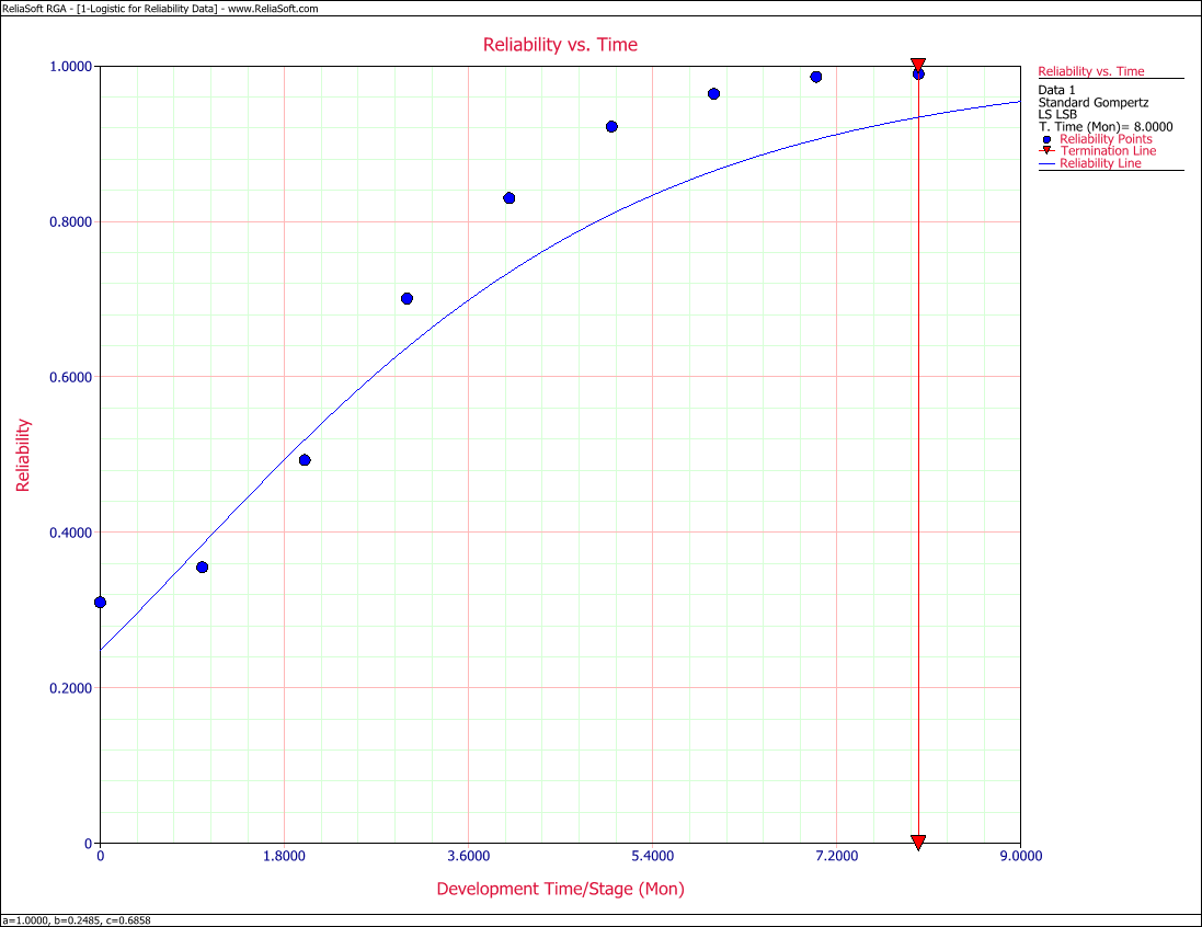
The values of predicted reliabilities are plotted in Figure Logig81.
[math]\displaystyle{ }[/math]
Notice how the Standard Gompertz model is not really capable of handling the S-shaped characteristics of this data.
2. The least squares estimators of the Logistic growth curve parameters are [9]:
where:
- [math]\displaystyle{ \begin{align} & {{{\hat{b}}}_{1}}= & \frac{\underset{i=0}{\overset{N-1}{\mathop{\sum }}}\,{{T}_{i}}{{Y}_{i}}-N\cdot \bar{T}\cdot \bar{Y}}{\underset{i=0}{\overset{N-1}{\mathop{\sum }}}\,T_{i}^{2}-N\cdot {{{\bar{T}}}^{2}}} \\ & {{{\hat{b}}}_{0}}= & \bar{Y}-{{{\hat{b}}}_{1}}\bar{T} \\ & {{Y}_{i}}= & \ln \left( \frac{1}{{{R}_{i}}}-1 \right) \\ & \bar{Y}= & \frac{1}{N}\underset{i=0}{\overset{N-1}{\mathop \sum }}\,{{Y}_{i}} \end{align} }[/math]
In this example [math]\displaystyle{ N=9 }[/math] , which gives:
From Eqns. (eq37) and (eq38):
And from Eqns. (eq36a) and (eq36b):
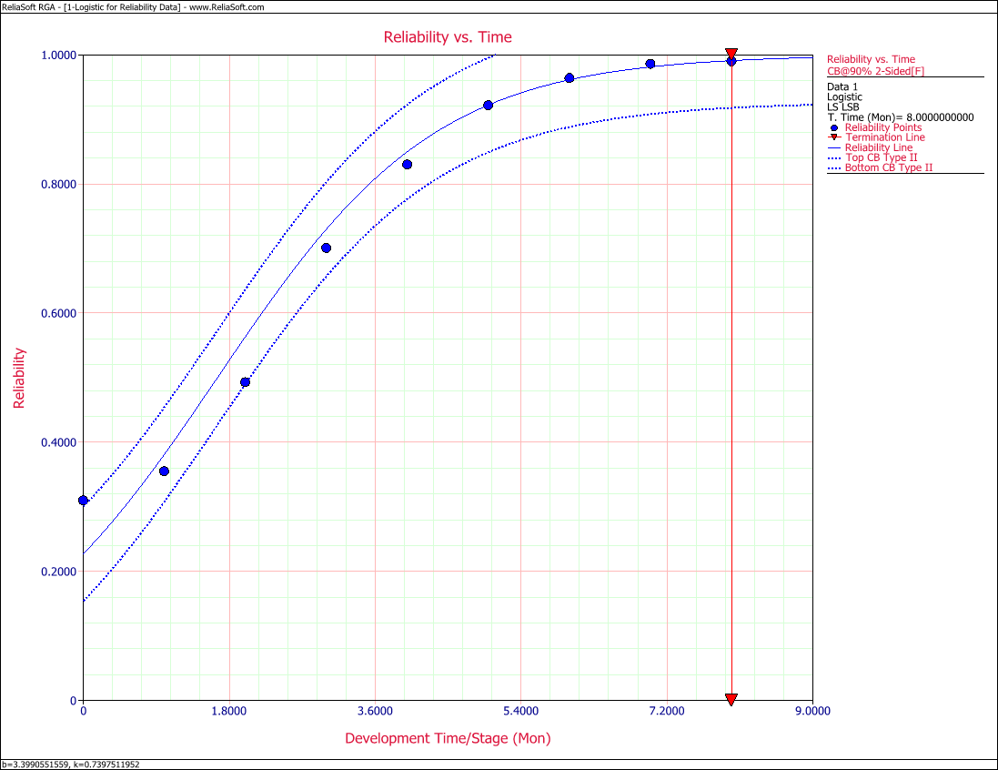
- [math]\displaystyle{ \begin{align} & \widehat{b}= & {{e}^{1.2235}} \\ & = & 3.3991 \\ & \widehat{k}= & -(-0.7398) \\ & = & 0.7398 \end{align} }[/math]
Therefore, the Logistic reliability growth curve that represents this data set is given by:
- [math]\displaystyle{ R=\frac{1}{1+3.3991\,{{e}^{-0.7398\,T}}} }[/math]
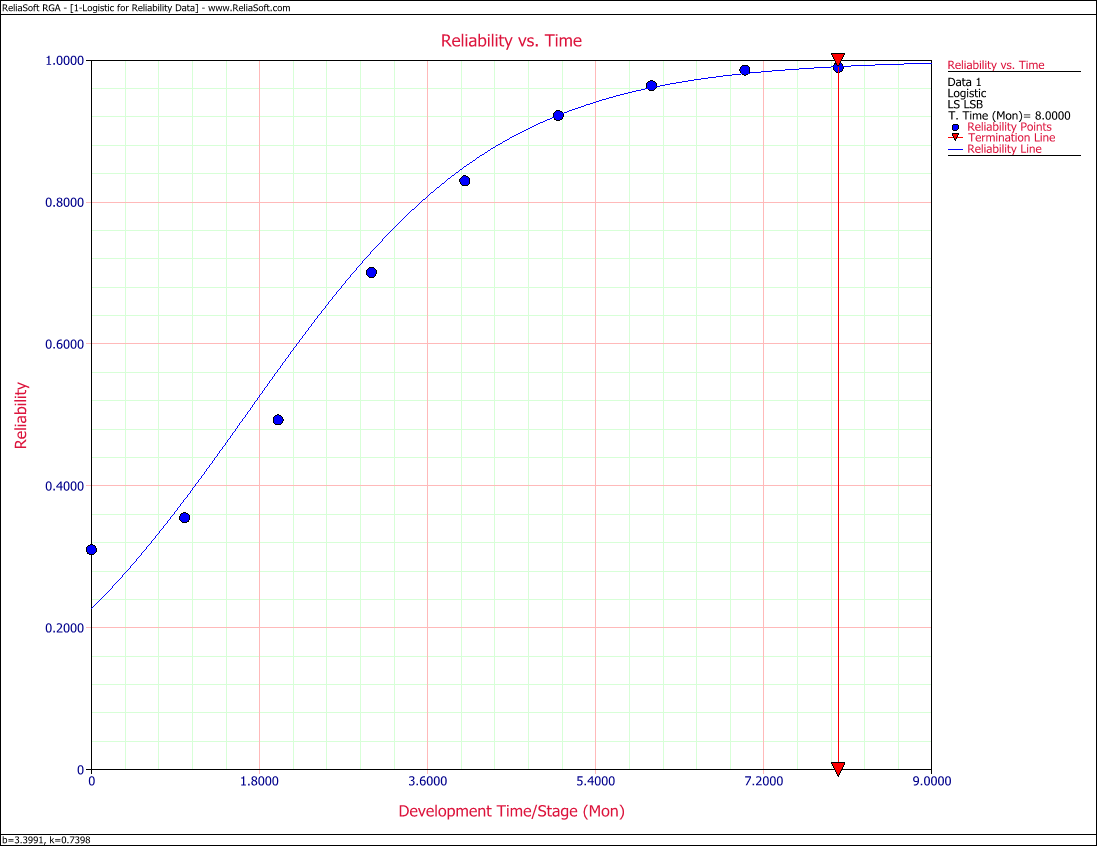
Figure Logig82 shows the Reliability vs. Time plot. The plot shows that the observed data set is estimated well by the Logistic reliability growth curve, except in the region closely surrounding the inflection point of the observed reliability. This problem can be overcome by using the Modified Gompertz model, which was presented in Chapter 7.
Example 2
A prototype was tested under a success/failure pattern. The test consisted of 15 runs and Table 8.2 presents the data from the test. Find the Logistic model that best fits the data set and plot it along with the reliability observed from the raw data.
| Time | Result | Observed Reliability |
|---|---|---|
| 0 | F | 0.5000 |
| 1 | F | 0.3333 |
| 2 | S | 0.5000 |
| 3 | S | 0.6000 |
| 4 | F | 0.5000 |
| 5 | S | 0.5714 |
| 6 | S | 0.6250 |
| 7 | S | 0.6667 |
| 8 | S | 0.7000 |
| 9 | F | 0.6364 |
| 10 | S | 0.6667 |
| 11 | S | 0.6923 |
| 12 | S | 0.7143 |
| 13 | S | 0.7333 |
Solution
The first run is ignored because it was a success and the reliability at that point was 100%. This failure will be ignored throughout the analysis because it is considered that the test starts when the reliability is not equal to zero or one. The test essentially begins at time 1, and is now considered as time 0 with [math]\displaystyle{ N=14 }[/math] . The observed reliability is shown in the last column of Table 8.2. Keep in mind that the observed reliability values still account for the initial suspension.
Eqn. (eq41a) becomes:
- [math]\displaystyle{ \begin{align} & \bar{Y}= & \frac{1}{N}\underset{i=0}{\overset{N-1}{\mathop \sum }}\,{{Y}_{i}} \\ & = & \frac{1}{14}\underset{i=0}{\overset{13}{\mathop \sum }}\,\ln \left( \frac{1}{{{R}_{i}}}-1 \right) \\ & = & -0.43163 \end{align} }[/math]
and:
- [math]\displaystyle{ \begin{align} & \bar{T}= & \frac{1}{14}\underset{i=0}{\overset{13}{\mathop \sum }}\,{{T}_{i}} \\ & = & 6.5 \\ & \underset{i=0}{\overset{13}{\mathop \sum }}\,T_{i}^{2}= & 819.0 \\ & \underset{i=0}{\overset{13}{\mathop \sum }}\,{{T}_{i}}{{Y}_{i}}= & -61.69 \end{align} }[/math]
Now, from the least squares estimators, Eqns. (eq37) and (eq38) are:
Therefore:
- [math]\displaystyle{ \begin{align} & \widehat{b}= & {{e}^{0.2087}} \\ & = & 1.2321 \\ & \widehat{k}= & -(-0.0985) \\ & = & 0.0985 \end{align} }[/math]
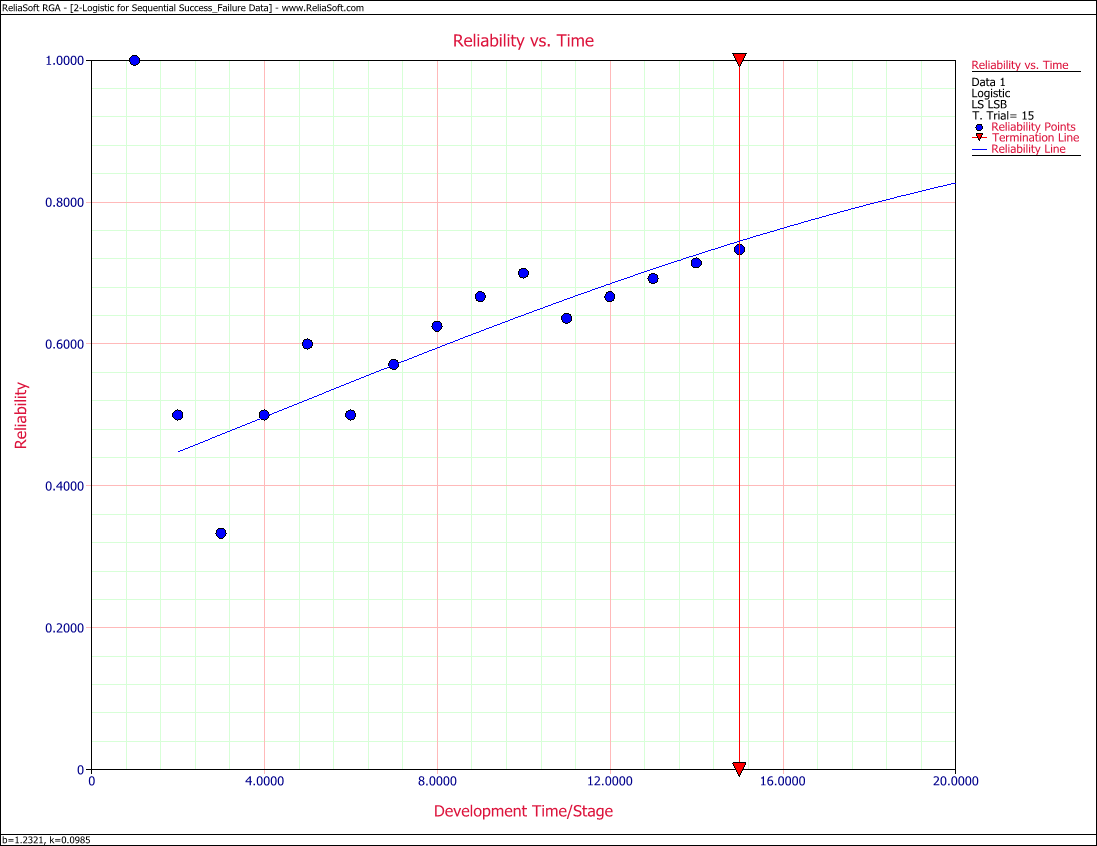
The Logistic reliability model that best fits the data is given by:
- [math]\displaystyle{ R=\frac{1}{1+1.2321\cdot \ \,{{e}^{-0.0985T}}} }[/math]
Figure Logig83 shows the Reliability vs. Time plot.
Example 3
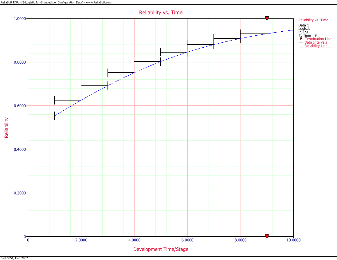
Some equipment underwent testing in different stages. The testing may have been performed in subsequent days, weeks or months with an unequal number of units tested every day. Each group was tested and several failures occurred. The data set is given in columns 1 and 2 of Table 8.3. Find the Logistic model that best fits the data and plot it along with the reliability observed from the raw data.
| Number of Units | Number of Failures | [math]\displaystyle{ T_i }[/math] | Observed Reliability |
|---|---|---|---|
| 10 | 5 | 0 | 0.5000 |
| 8 | 3 | 1 | 0.6250 |
| 9 | 3 | 2 | 0.6667 |
| 9 | 2 | 3 | 0.7778 |
| 10 | 2 | 4 | 0.8000 |
| 10 | 1 | 5 | 0.9000 |
| 10 | 1 | 6 | 0.9000 |
| 10 | 1 | 7 | 0.9000 |
| 10 | 1 | 8 | 0.9000 |
Solution
The observed reliability is [math]\displaystyle{ 1-\tfrac{\#\text{ of failures}}{\#\text{ of units}} }[/math] and the last column of Table 8.3 shows the values for each group. With [math]\displaystyle{ N=9 }[/math] , Eqn. (eq41a) becomes:
- [math]\displaystyle{ \begin{align} & \bar{Y}= & \frac{1}{9}\underset{i=0}{\overset{8}{\mathop \sum }}\,\ln \left( \frac{1}{{{R}_{i}}}-1 \right) \\ & = & -1.4036 \end{align} }[/math]
and:
- [math]\displaystyle{ \begin{align} & \bar{T}= & \frac{1}{9}\underset{i=0}{\overset{8}{\mathop \sum }}\,{{T}_{i}} \\ & = & 4 \\ & \underset{i=0}{\overset{8}{\mathop \sum }}\,T_{i}^{2}= & 204 \\ & \underset{i=0}{\overset{8}{\mathop \sum }}\,{{T}_{i}}{{Y}_{i}}= & -68.33 \end{align} }[/math]
Now from the least squares estimators, Eqns. (eq37) and (eq38) give:
- [math]\displaystyle{ \begin{align} & {{{\hat{b}}}_{1}}= & \frac{\underset{i=0}{\overset{8}{\mathop{\sum }}}\,{{T}_{i}}{{Y}_{i}}-N\cdot \bar{T}\cdot \bar{Y}}{\underset{i=0}{\overset{8}{\mathop{\sum }}}\,T_{i}^{2}-N\cdot {{{\bar{T}}}^{2}}} \\ & = & \frac{-68.33-9\cdot 4\cdot \left( -1.4036 \right)}{204-9\cdot {{4}^{2}}} \\ & = & -0.2967 \\ & & \\ & {{{\hat{b}}}_{0}}= & \bar{Y}-{{{\hat{b}}}_{1}}\bar{T} \\ & = & \left( -1.4036 \right)-\left( -0.2967 \right)\cdot 4.0 \\ & = & -0.2168 \end{align} }[/math]
Therefore:
- [math]\displaystyle{ \begin{align} & \widehat{b}= & {{e}^{-0.2168}} \\ & = & 0.8051 \\ & \widehat{k}= & -(-0.2967) \\ & = & 0.2967 \end{align} }[/math]
The Logistic reliability model that best fits the data is given by:
- [math]\displaystyle{ R=\frac{1}{1+0.8051\cdot \ \,{{e}^{-0.2967T}}} }[/math]
Figure Logig85 shows the Reliability vs. Time plot.
[math]\displaystyle{ }[/math]
Confidence Bounds
Least squares is used to estimate the parameters of the following Logistic model.
- [math]\displaystyle{ \ln (\frac{1}{{{{\hat{R}}}_{i}}}-1)=\ln (b)-k{{T}_{i}} }[/math]
Thus the confidence bounds on the parameters are given by:
- [math]\displaystyle{ b=\hat{b}{{e}^{{{t}_{n-2,\alpha /2}}SE(\ln \hat{b})}} }[/math]
where:
- [math]\displaystyle{ SE(\ln \hat{b})=\sigma \cdot \sqrt{\frac{\underset{i=1}{\overset{n}{\mathop{\sum }}}\,{{({{T}_{i}})}^{2}}}{n\cdot {{S}_{xx}}}},\ \ \ {{S}_{xx}}=\left[ \underset{i=1}{\overset{n}{\mathop \sum }}\,{{({{T}_{i}})}^{2}} \right]-\frac{1}{n}{{\left( \underset{i=1}{\overset{n}{\mathop \sum }}\,{{T}_{i}} \right)}^{2}} }[/math]
- [math]\displaystyle{ \sigma =\sqrt{SSE/(n-2)} }[/math]
and:
- [math]\displaystyle{ k=\hat{k}\pm {{t}_{n-2,\alpha /2}}SE(\hat{k}) }[/math]
where:
- [math]\displaystyle{ SE(\hat{k})=\frac{\sigma }{\sqrt{{{S}_{xx}}}},\ \ {{S}_{xx}}=\left[ \underset{i=1}{\overset{n}{\mathop \sum }}\,{{({{T}_{i}})}^{2}} \right]-\frac{1}{n}{{\left( \underset{i=1}{\overset{n}{\mathop \sum }}\,{{T}_{i}} \right)}^{2}} }[/math]
Since the reliability is always between 0 and 1, the logit transformation is used to obtain the confidence bounds on reliability.
- [math]\displaystyle{ CB=\frac{{{{\hat{R}}}_{i}}}{{{{\hat{R}}}_{i}}+(1-{{{\hat{R}}}_{i}}){{e}^{\pm {{z}_{\alpha }}{{{\hat{\sigma }}}_{R}}/\left[ {{{\hat{R}}}_{i}}(1-{{{\hat{R}}}_{i}}) \right]}}} }[/math]
Example 4
For the data given for Example 1 in Table 8.1, calculate the 2-sided 90% confidence bounds under the Logistic model for the following:
1) The parameters [math]\displaystyle{ b }[/math] and [math]\displaystyle{ k }[/math] .
2) Reliability at month 5.
Solution
1) The values of [math]\displaystyle{ \widehat{b} }[/math] and [math]\displaystyle{ \widehat{k} }[/math] estimated from the least squares analysis in Example 1:
- [math]\displaystyle{ \begin{align} & \widehat{b}= & 3.3991 \\ & \widehat{\alpha }= & 0.7398 \end{align} }[/math]
Thus the 2-sided 90% confidence bounds on parameter [math]\displaystyle{ b }[/math] using Eqn. (LogCBb) are:
- [math]\displaystyle{ \begin{align} & {{b}_{lower}}= & 2.5547 \\ & {{b}_{upper}}= & 4.5225 \end{align} }[/math]
The 2-sided 90% confidence bounds on parameter [math]\displaystyle{ k }[/math] using Eqn. (logCBk) are:
- [math]\displaystyle{ \begin{align} & {{k}_{lower}}= & 0.6798 \\ & {{k}_{upper}}= & 0.7997 \end{align} }[/math]
2) First calculate the reliability estimation at month 5:
- [math]\displaystyle{ \begin{align} & {{R}_{5}}= & \frac{1}{1+b{{e}^{-5k}}} \\ & = & 0.9224 \end{align} }[/math]
Thus the 2-sided 90% confidence bounds on reliability at month 5 using Eqn. (LogCR) are:
- [math]\displaystyle{ \begin{align} & {{[{{R}_{5}}]}_{lower}}= & 0.8493 \\ & {{[{{R}_{5}}]}_{upper}}= & 0.9955 \end{align} }[/math]
Figure Logig86 shows a graph of the reliability plotted with 2-sided 90% confidence bounds.
[math]\displaystyle{ }[/math]
General Examples
Example 5
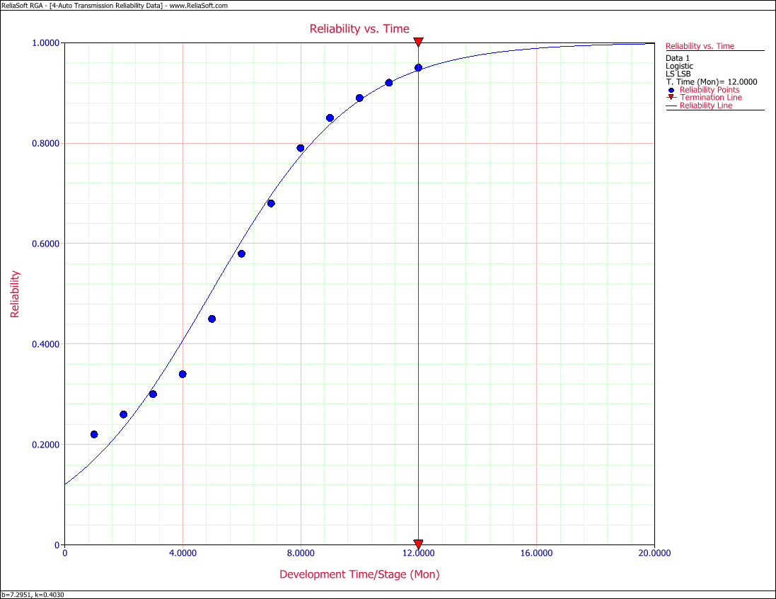
Table 8.4 presents the reliabilities observed monthly for an automobile transmission that was tested for one year.
1) Find a Logistic reliability growth curve that best represents the data.
2) Plot it comparatively with the raw data.
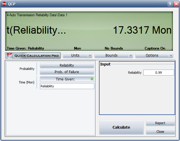
3) If design changes continue to be incorporated and the testing continues, when will the reliability goal of 99% be achieved?
4) If design changes continue to be incorporated and the testing continues, what will be the attainable reliability at the end of January the following year?
| Month | Observed Reliability(%) |
|---|---|
| June | 22 |
| July | 26 |
| August | 30 |
| September | 34 |
| October | 45 |
| November | 58 |
| December | 68 |
| January | 79 |
| February | 85 |
| March | 89 |
| April | 92 |
| May | 95 |
Solution to Example 5
1) Figure Loge21 shows the estimated parameters.
2) Figure Loge22 displays the Reliability vs. Time plot.
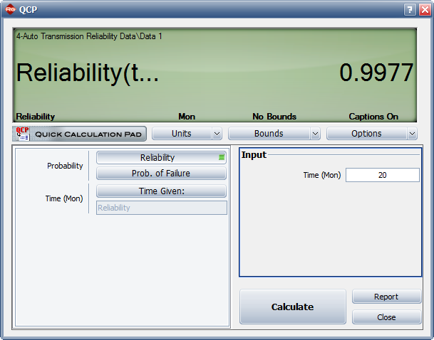
3) Using the QCP, Figure Loge23 displays when the reliability goal of 99% will be achieved.
4) Figure Loge24 shows the reliability at the end of January the following year (i.e. after 20 months of testing and development).
Example 6
Table 8.5 presents the results for a missile launch test. The test consisted of 20 attempts. If the missile launched, it was recorded as a success. If not, it was recorded as a failure. Note that, at this development stage, the test did not consider whether or not the target was destroyed.
1) Find a Logistic reliability growth curve that best represents the data.
2) Plot it comparatively with the raw data.
3) If design changes continue to be incorporated and the testing continues, when will the reliability goal of 99.5% with a 90% confidence level be achieved?
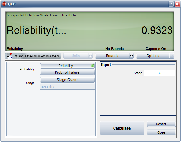
4) If design changes continue to be incorporated and the testing continues, what will be the attainable reliability at the end of the 35th launch?
| Launch Number | Result |
|---|---|
| 1 | F |
| 2 | F |
| 3 | S |
| 4 | F |
| 5 | F |
| 6 | S |
| 7 | S |
| 8 | S |
| 9 | F |
| 10 | S |
| 11 | F |
| 12 | S |
| 13 | S |
| 14 | S |
| 15 | S |
| 16 | S |
| 17 | S |
| 18 | S |
| 19 | S |
| 20 | S |
Solution to Example 6
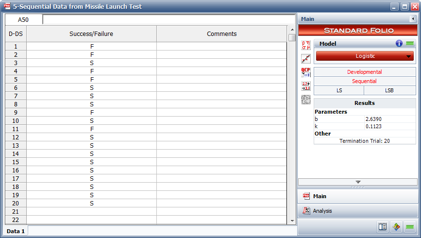
1) Figure Loge31 shows the entered data and the estimated parameters.
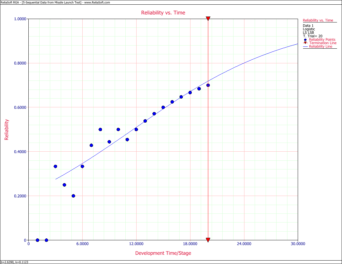
2) Figure Loge32 displays the Reliability vs. Time plot.
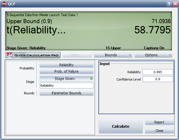
3) Figure Loge33 displays when the reliability goal of 99.5% will be achieved with a 90% confidence level.
4) Figure Loge34 displays the reliability achieved after the 35th launch.
[math]\displaystyle{ }[/math]
Example 7
Consider the data given for the missile launch test in Example 6. Now suppose that the engineers assigned failure modes to each failure and that the appropriate corrective actions were taken.
Table 8.6 presents the data.
1) Find the Logistic reliability growth curve that best represents the data.
2) Plot it comparatively with the raw data.
3) If design changes continue to be incorporated and the testing continues, when will the reliability goal of 99.50% be achieved?
4) If design changes continue to be incorporated and the testing continues, what will be the attainable reliability at the end of the 35th launch?
| Launch Number | Result | Mode |
|---|---|---|
| 1 | F | 2 |
| 2 | F | 1 |
| 3 | S | |
| 4 | F | 3 |
| 5 | F | 3 |
| 6 | S | |
| 7 | S | |
| 8 | S | |
| 9 | F | 2 |
| 10 | S | |
| 11 | F | 1 |
| 12 | S | |
| 13 | S | |
| 14 | S | |
| 15 | S | |
| 16 | S | |
| 17 | S | |
| 18 | S | |
| 19 | S | |
| 20 | S |
Solution to Example 7
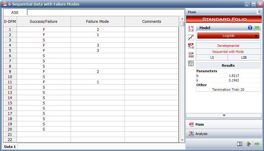
1) Figure Loge51 shows the estimated parameters.
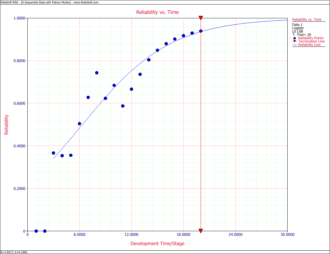
2) Figure Loge52 displays the Reliability vs. Time plot.
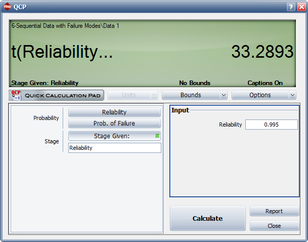
3) Figure Loge53 displays when the reliability goal of 99.5% will be achieved.
4) Figure Loge54 displays the reliability after the 35th launch.
[math]\displaystyle{ }[/math]
- Figure 8.16: Reliability vs. Time plot.

