Optimal Test Plan for Two Stresses: Difference between revisions
Jump to navigation
Jump to search
Kate Racaza (talk | contribs) No edit summary |
Kate Racaza (talk | contribs) No edit summary |
||
| Line 49: | Line 49: | ||
{{Reference_Example_Heading4|ALTA}} | {{Reference_Example_Heading4|ALTA}} | ||
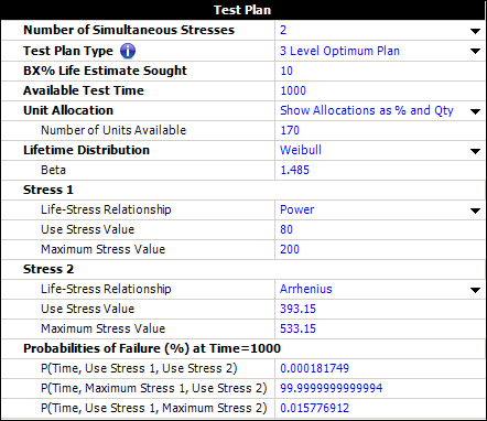
The planning information is entered in ALTA as shown below. | The planning information is entered in ALTA, as shown below. | ||
[[Image:Optimal plan 2 stresses.png|center]] | |||
The probabilities of failure (%) at time of 1000 are calculated based on test planning values. For example, at the use stress of voltage and at the maximum stress of temperature, the life characteristic is: | |||
::<math>\begin{align} | |||
ln(\eta) =& \beta_{0}+\beta_{1} \times log(vpm) + \beta_{2} \frac{11605}{temp} \\ | |||
=& 58.173 - 12.28 \times ln(80) + 0.3878 \frac{11605}{533.15}\\ | |||
=& 12.8029 | |||
\end{align}\,\!</math> | |||
Therefore, <math>\eta\,\!</math> = 363269. The probability of failure is calculated by: | |||
::<math>\begin{align} | |||
P(Time, Use Stress 1, Maximum Stress 2) =& P(1000, 80, 533.15)\\ | |||
=& 1 - e^{-\left(\frac{1000}{363269} \right)^{1.485}}\\ | |||
=& 0.000158 = 0.0158% | |||
\end{align}\,\!</math> | |||
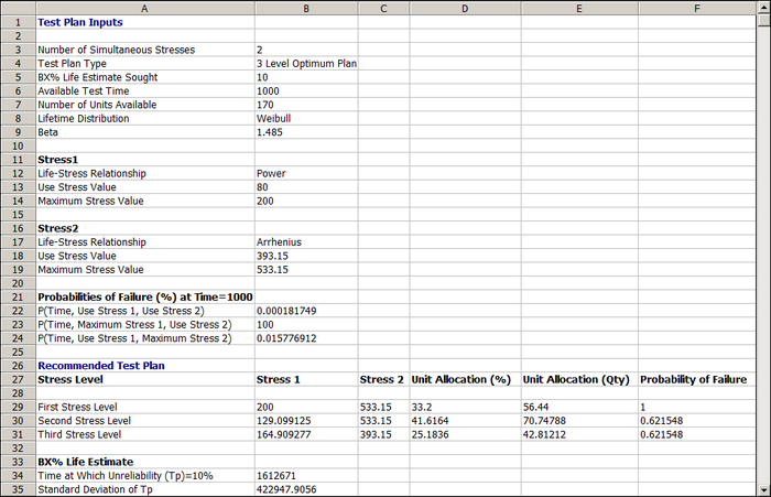
The three level best compromise test plan in ALTA is shown below. | |||
[[Image: Optimal plan test plan.png|center|700px]] | |||
The test plan shows that: | |||
* The first stress level (row 29) should be a combination of 200 volts and 260°C (533.15°K) and about 56 units should be tested at that level. | |||
* The second stress level (row 30) should be a combination of 129 volts and 260°C (533.15°K) and about 71 units should be tested at that level. | |||
* The third stress level (row 31) should be a combination of 165 volts and 120°C (393.15°K) and about 43 units should be tested at that level. | |||
The estimated standard deviation of the log B10 life at 50°C can be obtained by: | |||
::<math>Ase \left[ log \left(\hat{t}_{0.1}(50) \right)\right] = \frac{Ase\left(\hat{t}_{0.1}(50) \right)}{\hat{t}_{0.1}(50)} = \frac{422947.9056}{1612671} = 0.262265\,\!</math> | |||
The above results are different from the results given in the book. In the following discussion, a simulation study is conducted to check the results obtained from ALTA. | |||
'''Using ALTA SimuMatic to Evaluate the Test Plan''' | |||
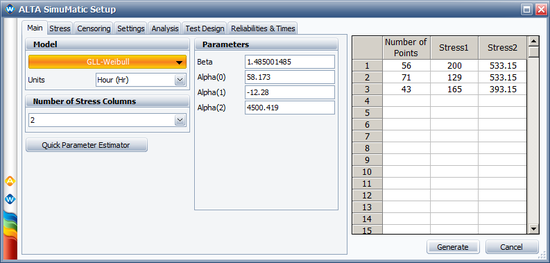
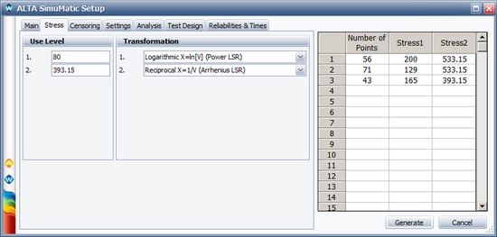
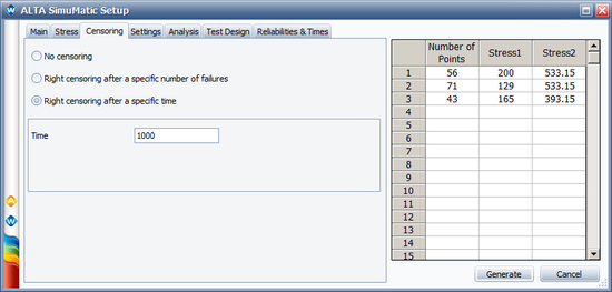
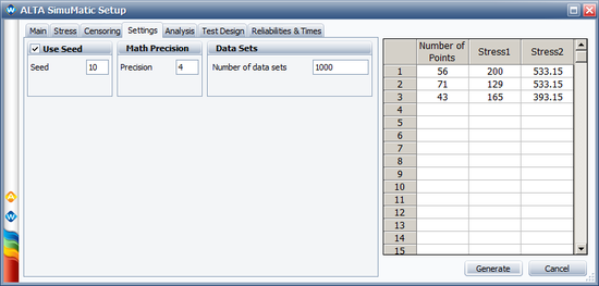
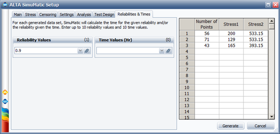
We will use the SimuMatic utility to evaluate the test plan. The following pictures show the settings used in SimuMatic (with <math>\alpha_{1} = \beta_{1} \times 11605\,\!</math>): | |||
[[Image: Optimal plan simumatic1.png|center|550px]] | |||
[[Image: Optimal plan simumatic2.png|center|550px]] | |||
[[Image: Optimal plan simumatic3.png|center|550px]] | |||
[[Image: Optimal plan simumatic4.png|center|550px]] | |||
[[Image: Optimal plan simumatic5.png|center|550px]] | |||
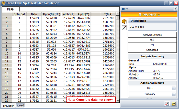
The simulation results are shown next. | |||
[[Image: Optimal plan simumatic6.png|center|700px]] | |||
We take the nature log of the B10 life (the last column) and calculate its standard deviation. The calculated standard deviation is 0.2629. This is very close to the analytical solution from the ALTA test plan tool, where the standard deviation is 0.2623. | |||
This standard deviation is smaller than the standard deviation given by the test plan in the book. Therefore, the test plan generated in ALTA is better than the test plan given in the book in terms of minimizing the estimation variance of the B10 life. | |||
Revision as of 16:15, 11 June 2014
ALTA_Reference_Examples_Banner.png
