ANOVA for Designed Experiments: Difference between revisions
No edit summary |
|||
| Line 1,619: | Line 1,619: | ||
<br> | <br> | ||
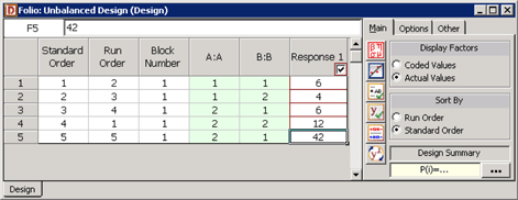
::Figure 6.15: Unbalanced experimental design for the data in Table 6.6. | ::Figure 6.15: Unbalanced experimental design for the data in Table 6.6. | ||
[[File:doe6.16.png|center]] | |||
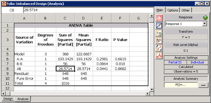
::Figure 6.16: Analysis for the unbalanced data in Table 6.6. | |||
Revision as of 16:19, 8 July 2011
Analysis of Experiments
Introduction
In Chapters 4 and 5, methods were presented to model the relationship between a response and the associated factors (referred to as predictor variables in the context of regression) based on an observed data set. Such studies, where observed values of the response are used to establish an association between the response and the factors, are called observational studies. However, in the case of observational studies, it is difficult to establish a cause-and-effect relationship between the observed factors and the response. This is because a number of alternative justifications can be used to explain the observed change in the response values. For example, a regression model fitted to data on the population of cities and road accidents might show a positive regression relation. However, this relation does not imply that an increase in a city's population causes an increase in road accidents. It could be that a number of other factors such as road conditions, traffic control and the degree to which the residents of the city follow the traffic rules affect the number of road accidents in the city and the increase in the number of accidents seen in the study is caused by these factors. Since the observational study does not take the effect of these factors into account, the assumption that an increase a city's population will lead to an increase in road accidents is not a valid one. For example, the population of a city may increase but road accidents in the city may decrease because of better traffic control. To establish a cause-and-effect relationship, the study should be conducted in such a way that the effect of all other factors is excluded from the investigation. The studies that enable the establishment of a cause-and-effect relationship are called experiments. In experiments the response is investigated by studying only the effect of the factor(s) of interest and excluding all other effects that may provide alternative justifications to the observed change in response. This is done in two ways. First, the levels of the factors to be investigated are carefully selected and then strictly controlled during the execution of the experiment. The aspect of selecting what factor levels should be investigated in the experiment is called the design of the experiment. The second distinguishing feature of experiments is that observations in an experiment are recorded in a random order. By doing this, it is hoped that the effect of all other factors not being investigated in the experiment will get cancelled out so that the change in the response is the result of only the investigated factors. Using these two techniques, experiments tend to ensure that alternative justifications to observed changes in the response are voided, thereby enabling the establishment of a cause-and-effect relationship between the response and the investigated factors.
Randomization
The aspect of recording observations in an experiment in a random order is referred to as randomization. Specifically randomization is the process of assigning the various levels of the investigated factors to the experimental units in a random fashion. An experiment is said to be completely randomized if the probability of an experimental unit to be subjected to any level of a factor is equal for all the experimental units. The importance of randomization can be illustrated using an example. Consider an experiment where the effect of the speed of a lathe machine on the surface finish of a product is being investigated. In order to save time, the experimenter records surface finish values by running the lathe machine continuously and recording observations in the order of increasing speeds. The analysis of the experiment data shows that an increase in lathe speeds causes a decrease in the quality of surface finish. However the results of the experiment are disputed by the lathe operator who claims that he has been able to obtain better surface finish quality in the products by operating the lathe machine at higher speeds. It is later found that the faulty results were caused because of over heating of the tool used in the machine. Since the lathe was run continuously in the order of increased speeds the observations were recorded in the order of increased tool temperatures. This problem could have been avoided if the experimenter had randomized the experiment and taken reading at the various lathe speeds in a random fashion. This would require the experimenter to stop and restart the machine at every observation, thereby keeping the temperature of the tool within a reasonable range. Randomization would have ensured that the effect of heating of the machine tool is not included in the experiment.
Analysis of Single Factor Experiments
As explained in Chapters 4 and 5, the analysis of observational studies involves the use of regression models. The analysis of experimental studies involves the use of analysis of variance (ANOVA) models. For a comparison of the two models see Section 6.SingleFactAnalysis. In single factor experiments, ANOVA models are used to compare the mean response values at different levels of the factor. Each level of the factor is investigated to see if the response is significantly different from the response at other levels of the factor. The analysis of single factor experiments is often referred to as one-way ANOVA.
To illustrate the use of ANOVA models in the analysis of experiments, consider a single factor experiment where the analyst wants to see if the surface finish of certain parts is affected by the speed of a lathe machine. Data is collected for three speeds (or three treatments). Each treatment is replicated four times. Therefore, this experiment design is balanced. Surface finish values recorded using randomization are shown in Table 6.1.
- Figure 6.1: Surface finish values for three speeds of a lathe machine.
The ANOVA model for this experiment can be stated as follows:
- [math]\displaystyle{ {{Y}_{ij}}={{\mu }_{i}}+{{\epsilon }_{ij}} }[/math]
The ANOVA model assumes that the response at each factor level, [math]\displaystyle{ i }[/math] , is the sum of the mean response at the [math]\displaystyle{ i }[/math] th level, [math]\displaystyle{ {{\mu }_{i}} }[/math] , and a random error term, [math]\displaystyle{ {{\epsilon }_{ij}} }[/math] . The subscript [math]\displaystyle{ i }[/math] denotes the factor level while the subscript [math]\displaystyle{ j }[/math] denotes the replicate. If there are [math]\displaystyle{ {{n}_{a}} }[/math] levels of the factor and [math]\displaystyle{ m }[/math] replicates at each level then [math]\displaystyle{ i=1,2,...,{{n}_{a}} }[/math] and [math]\displaystyle{ j=1,2,...,m }[/math] . The random error terms, [math]\displaystyle{ {{\epsilon }_{ij}} }[/math] , are assumed to be normally and independently distributed with a mean of zero and variance of [math]\displaystyle{ {{\sigma }^{2}} }[/math] . Therefore, the response at each level can be thought of as a normally distributed population with a mean of [math]\displaystyle{ {{\mu }_{i}} }[/math] and constant variance of [math]\displaystyle{ {{\sigma }^{2}} }[/math] . Eqn. (MeansModel) is referred to as the means model.
The ANOVA model of Eqn. (MeansModel) can also be written using [math]\displaystyle{ {{\mu }_{i}}=\mu +{{\tau }_{i}} }[/math] , where [math]\displaystyle{ \mu }[/math] represents the overall mean and [math]\displaystyle{ {{\tau }_{i}} }[/math] represents the effect due to the [math]\displaystyle{ i }[/math] th treatment.
- [math]\displaystyle{ {{Y}_{ij}}=\mu +{{\tau }_{i}}+{{\epsilon }_{ij}} }[/math]
Such an ANOVA model is called the effects model. In the effects models the treatment effects, [math]\displaystyle{ {{\tau }_{i}} }[/math] , represent the deviations from the overall mean, [math]\displaystyle{ \mu }[/math] . Therefore, the following constraint exists on the [math]\displaystyle{ {{\tau }_{i}} }[/math] s:
- [math]\displaystyle{ \underset{i=1}{\overset{{{n}_{a}}}{\mathop \sum }}\,{{\tau }_{i}}=0 }[/math]
Fitting ANOVA Models
To fit ANOVA models and carry out hypothesis testing in single factor experiments, it is convenient to express the effects model of Eqn. (1factAnovaModel) in the form [math]\displaystyle{ y=X\beta +\epsilon }[/math] (that was used for multiple linear regression models in Chapter 5). This can be done as shown next. Using Eqn. (1factAnovaModel), the ANOVA model for the single factor experiment in Table 6.1 can be expressed as:
- [math]\displaystyle{ {{Y}_{ij}}=\mu +{{\tau }_{i}}+{{\epsilon }_{ij}} }[/math]
where [math]\displaystyle{ \mu }[/math] represents the overall mean and [math]\displaystyle{ {{\tau }_{i}} }[/math] represents the [math]\displaystyle{ i }[/math] th treatment effect. There are three treatments in Table 6.1 (500, 600 and 700). Therefore, there are three treatment effects, [math]\displaystyle{ {{\tau }_{1}} }[/math] , [math]\displaystyle{ {{\tau }_{2}} }[/math] and [math]\displaystyle{ {{\tau }_{3}} }[/math] . Per Eqn. (TreatmentEffectConstraint), the following constraint exists for these effects:
- [math]\displaystyle{ \begin{align} & \underset{i=1}{\overset{3}{\mathop \sum }}\,{{\tau }_{i}}= & 0 \\ & \text{or }{{\tau }_{1}}+{{\tau }_{2}}+{{\tau }_{3}}= & 0 \end{align} }[/math]
For the first treatment, Eqn. (AnovaModelSingleFactEx) can be written as:
- [math]\displaystyle{ {{Y}_{1j}}=\mu +{{\tau }_{1}}+0\cdot {{\tau }_{2}}+0\cdot {{\tau }_{3}}+{{\epsilon }_{1j}} }[/math]
Using [math]\displaystyle{ {{\tau }_{3}}=-({{\tau }_{1}}+{{\tau }_{2}}) }[/math] from Eqn. (ConstraintSingleFactEx), the model for the first treatment is:
- [math]\displaystyle{ \begin{align} & {{Y}_{1j}}= & \mu +{{\tau }_{1}}+0\cdot {{\tau }_{2}}-0\cdot ({{\tau }_{1}}+{{\tau }_{2}})+{{\epsilon }_{1j}} \\ & \text{or }{{Y}_{1j}}= & \mu +{{\tau }_{1}}+0\cdot {{\tau }_{2}}+{{\epsilon }_{1j}} \end{align} }[/math]
Models for the second and third treatments can be obtained in a similar way. The models for the three treatments are:
- [math]\displaystyle{ \begin{align} & \text{First Treatment}: & {{Y}_{1j}}=1\cdot \mu +1\cdot {{\tau }_{1}}+0\cdot {{\tau }_{2}}+{{\epsilon }_{1j}} \\ & \text{Second Treatment}: & {{Y}_{2j}}=1\cdot \mu +0\cdot {{\tau }_{1}}+1\cdot {{\tau }_{2}}+{{\epsilon }_{2j}} \\ & \text{Third Treatment}: & {{Y}_{3j}}=1\cdot \mu -1\cdot {{\tau }_{1}}-1\cdot {{\tau }_{2}}+{{\epsilon }_{3j}} \end{align} }[/math]
The coefficients of the treatment effects [math]\displaystyle{ {{\tau }_{1}} }[/math] and [math]\displaystyle{ {{\tau }_{2}} }[/math] in Eqns. (ExAnovaModelEq1) to (ExAnovalModelEq3) can be expressed using two indicator variables, [math]\displaystyle{ {{x}_{1}} }[/math] and [math]\displaystyle{ {{x}_{2}} }[/math] , as follows:
- [math]\displaystyle{ \begin{align} & \text{Treatment Effect }{{\tau }_{1}}: & {{x}_{1}}=1,\text{ }{{x}_{2}}=0 \\ & \text{Treatment Effect }{{\tau }_{2}}: & {{x}_{1}}=0,\text{ }{{x}_{2}}=1\text{ } \\ & \text{Treatment Effect }{{\tau }_{3}}: & {{x}_{1}}=-1,\text{ }{{x}_{2}}=-1\text{ } \end{align} }[/math]
Using the indicator variables [math]\displaystyle{ {{x}_{1}} }[/math] and [math]\displaystyle{ {{x}_{2}} }[/math] , the ANOVA model of Eqn. (AnovaModelSingleFactEx) for the data in Table 6.1 now becomes:
- [math]\displaystyle{ Y=\mu +{{x}_{1}}\cdot {{\tau }_{1}}+{{x}_{2}}\cdot {{\tau }_{2}}+\epsilon }[/math]
The equation can be rewritten by including subscripts [math]\displaystyle{ i }[/math] (for the level of the factor) and [math]\displaystyle{ j }[/math] (for the replicate number) as:
- [math]\displaystyle{ {{Y}_{ij}}=\mu +{{x}_{i1}}\cdot {{\tau }_{1}}+{{x}_{i2}}\cdot {{\tau }_{2}}+{{\epsilon }_{ij}} }[/math]
Eqn. (AnovaModelRegrVersion) represents the "regression version" of the ANOVA model.
Comparison of ANOVA and Regression Models
It can be seen from Eqn. (AnovaModelRegrVersion) that in an ANOVA model each factor is treated as a qualitative factor. In the present example the factor, lathe speed, is a quantitative factor with three levels. But the ANOVA model treats this factor as a qualitative factor with three levels. Therefore, two indicator variables, [math]\displaystyle{ {{x}_{1}} }[/math] and [math]\displaystyle{ {{x}_{2}} }[/math] , are required to represent this factor. Note that if a regression model were to be fitted to the data in Table 6.1 then a distinction is made between quantitative and qualitative factors. For regression models, the factor, lathe speed, would be used as a quantitative factor and represented with a single predictor variable. For example, if a first order regression model were to be fitted to the data in Table 6.1, then the regression model would take the form [math]\displaystyle{ {{Y}_{ij}}={{\beta }_{0}}+{{\beta }_{1}}{{x}_{i1}}+{{\epsilon }_{ij}} }[/math] . If a second order regression model were to be fitted, the regression model would be [math]\displaystyle{ {{Y}_{ij}}={{\beta }_{0}}+{{\beta }_{1}}{{x}_{i1}}+{{\beta }_{2}}x_{i1}^{2}+{{\epsilon }_{ij}} }[/math] . Notice that unlike these regression models, the ANOVA model of Eqn. (AnovaModelRegrVersion) does not make any assumption about the nature of relationship between the response and the factor being investigated.
The choice of the two models for a particular data set depends on the objective of the experimenter. In the case of the data of Table 6.1, the objective of the experimenter is to compare the levels of the factor to see if change in the levels leads to a significant change in the response. The objective is not to make predictions on the response for a given level of the factor. Therefore, the ANOVA model is used in this case. If the objective of the experimenter were prediction or optimization, the experimenter would use a regression model and focus on aspects such as the nature of relationship between the factor, lathe speed, and the response, surface finish, so that the regression model obtained is able to make accurate predictions.
Expression of the ANOVA Model in the Form [math]\displaystyle{ y=X\beta +\epsilon }[/math]
The ANOVA model of Eqn. (AnovaModelRegrVersion) can be expanded for the three treatments and four replicates of the data in Table 6.1 as follows:
- [math]\displaystyle{ \begin{align} & {{Y}_{11}}= & 6=\mu +1\cdot {{\tau }_{1}}+0\cdot {{\tau }_{2}}+{{\epsilon }_{11}}\text{ Level 1, Replicate 1} \\ & {{Y}_{21}}= & 13=\mu +0\cdot {{\tau }_{1}}+1\cdot {{\tau }_{2}}+{{\epsilon }_{21}}\text{ Level 2, Replicate 1} \\ & {{Y}_{31}}= & 23=\mu -1\cdot {{\tau }_{1}}-1\cdot {{\tau }_{2}}+{{\epsilon }_{31}}\text{ Level 3, Replicate 1} \\ & {{Y}_{12}}= & 13=\mu +1\cdot {{\tau }_{1}}+0\cdot {{\tau }_{2}}+{{\epsilon }_{12}}\text{ Level 1, Replicate 2} \\ & {{Y}_{22}}= & 16=\mu +0\cdot {{\tau }_{1}}+1\cdot {{\tau }_{2}}+{{\epsilon }_{22}}\text{ Level 2, Replicate 2} \\ & {{Y}_{32}}= & 20=\mu -1\cdot {{\tau }_{1}}-1\cdot {{\tau }_{2}}+{{\epsilon }_{32}}\text{ Level 3, Replicate 2} \\ & & ... \\ & {{Y}_{34}}= & 18=\mu -1\cdot {{\tau }_{1}}-1\cdot {{\tau }_{2}}+{{\epsilon }_{34}}\text{ Level 3, Replicate 4} \end{align} }[/math]
The corresponding matrix notation is:
- [math]\displaystyle{ y=X\beta +\epsilon }[/math]
where
- [math]\displaystyle{ y=\left[ \begin{matrix} {{Y}_{11}} \\ {{Y}_{21}} \\ {{Y}_{31}} \\ {{Y}_{12}} \\ {{Y}_{22}} \\ . \\ . \\ . \\ {{Y}_{34}} \\ \end{matrix} \right]=X\beta +\epsilon =\left[ \begin{matrix} 1 & 1 & 0 \\ 1 & 0 & 1 \\ 1 & -1 & -1 \\ 1 & 1 & 0 \\ 1 & 0 & 1 \\ . & . & . \\ . & . & . \\ . & . & . \\ 1 & -1 & -1 \\ \end{matrix} \right]\left[ \begin{matrix} \mu \\ {{\tau }_{1}} \\ {{\tau }_{2}} \\ \end{matrix} \right]+\left[ \begin{matrix} {{\epsilon }_{11}} \\ {{\epsilon }_{21}} \\ {{\epsilon }_{31}} \\ {{\epsilon }_{12}} \\ {{\epsilon }_{22}} \\ . \\ . \\ . \\ {{\epsilon }_{34}} \\ \end{matrix} \right] }[/math]
Thus:
- [math]\displaystyle{ \begin{align} & y= & X\beta +\epsilon \\ & & \\ & \left[ \begin{matrix} 6 \\ 13 \\ 23 \\ 13 \\ 16 \\ . \\ . \\ . \\ 18 \\ \end{matrix} \right]= & \left[ \begin{matrix} 1 & 1 & 0 \\ 1 & 0 & 1 \\ 1 & -1 & -1 \\ 1 & 1 & 0 \\ 1 & 0 & 1 \\ . & . & . \\ . & . & . \\ . & . & . \\ 1 & -1 & -1 \\ \end{matrix} \right]\left[ \begin{matrix} \mu \\ {{\tau }_{1}} \\ {{\tau }_{2}} \\ \end{matrix} \right]+\left[ \begin{matrix} {{\epsilon }_{11}} \\ {{\epsilon }_{21}} \\ {{\epsilon }_{31}} \\ {{\epsilon }_{12}} \\ {{\epsilon }_{22}} \\ . \\ . \\ . \\ {{\epsilon }_{34}} \\ \end{matrix} \right] \end{align} }[/math]
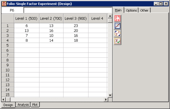
The matrices [math]\displaystyle{ y }[/math] , [math]\displaystyle{ X }[/math] and [math]\displaystyle{ \beta }[/math] are used in the calculation of the sum of squares in the next section. The data in Table 6.1 can be entered into DOE++ as shown in Figure SingleFactExSshot.
- Figure 6.1: Single factor experiment design for the data in Table 6.1.
Hypothesis Test in Single Factor Experiments
The hypothesis test in single factor experiments examines the ANOVA model to see if the response at any level of the investigated factor is significantly different from that at the other levels. If this is not the case and the response at all levels is not significantly different, then it can be concluded that the investigated factor does not affect the response. The test on the ANOVA model is carried out by checking to see if any of the treatment effects, [math]\displaystyle{ {{\tau }_{i}} }[/math] , are non-zero. The test is similar to the test of significance of regression mentioned in Chapters 4 and 5 in the context of regression models. The hypotheses statements for this test are:
- [math]\displaystyle{ \begin{align} & {{H}_{0}}: & {{\tau }_{1}}={{\tau }_{2}}=...={{\tau }_{{{n}_{a}}}}=0 \\ & {{H}_{1}}: & {{\tau }_{i}}\ne 0\text{ for at least one }i \end{align} }[/math]
The test for [math]\displaystyle{ {{H}_{0}} }[/math] is carried out using the following statistic:
- [math]\displaystyle{ {{F}_{0}}=\frac{M{{S}_{TR}}}{M{{S}_{E}}} }[/math]
where [math]\displaystyle{ M{{S}_{TR}} }[/math] represents the mean square for the ANOVA model and [math]\displaystyle{ M{{S}_{E}} }[/math] is the error mean square. Note that in the case of ANOVA models we use the notation [math]\displaystyle{ M{{S}_{TR}} }[/math] (treatment mean square) for the model mean square and [math]\displaystyle{ S{{S}_{TR}} }[/math] (treatment sum of squares) for the model sum of squares (instead of [math]\displaystyle{ M{{S}_{R}} }[/math] , regression mean square, and [math]\displaystyle{ S{{S}_{R}} }[/math] , regression sum of squares, used in Chapters 4 and 5). This is done to indicate that the model under consideration is the ANOVA model and not the regression model. The calculations to obtain [math]\displaystyle{ M{{S}_{TR}} }[/math] and [math]\displaystyle{ S{{S}_{TR}} }[/math] are identical to the calculations to obtain [math]\displaystyle{ M{{S}_{R}} }[/math] and [math]\displaystyle{ S{{S}_{R}} }[/math] explained in Chapter 5.
Calculation of the Statistic [math]\displaystyle{ {{F}_{0}} }[/math]
The sum of squares to obtain the statistic [math]\displaystyle{ {{F}_{0}} }[/math] can be calculated as explained in Chapter 5. Using the data in Table 6.1, the model sum of squares, [math]\displaystyle{ S{{S}_{TR}} }[/math] , can be calculated as:
- [math]\displaystyle{ \begin{align} & S{{S}_{TR}}= & {{y}^{\prime }}[H-(\frac{1}{{{n}_{a}}\cdot m})J]y \\ & = & {{\left[ \begin{matrix} 6 \\ 13 \\ . \\ . \\ 18 \\ \end{matrix} \right]}^{\prime }}\left[ \begin{matrix} 0.1667 & -0.0833 & . & . & -0.0833 \\ -0.0833 & 0.1667 & . & . & -0.0833 \\ . & . & . & . & . \\ . & . & . & . & . \\ -0.0833 & -0.0833 & . & . & 0.1667 \\ \end{matrix} \right]\left[ \begin{matrix} 6 \\ 13 \\ . \\ . \\ 18 \\ \end{matrix} \right] \\ & = & 232.1667 \end{align} }[/math]
In the previous equation, [math]\displaystyle{ {{n}_{a}} }[/math] represents the number of levels of the factor, [math]\displaystyle{ m }[/math] represents the replicates at each level, [math]\displaystyle{ y }[/math] represents the vector of the response values, [math]\displaystyle{ H }[/math] represents the hat matrix and [math]\displaystyle{ J }[/math] represents the matrix of ones. (For details on each of these terms, refer to Chapter 5.)
Since two effect terms, [math]\displaystyle{ {{\tau }_{1}} }[/math] and [math]\displaystyle{ {{\tau }_{2}} }[/math] , are used in the model of Eqn. (AnovaModelRegrVersion), the degrees of freedom associated with the model sum of squares, [math]\displaystyle{ S{{S}_{TR}} }[/math] , is two.
- [math]\displaystyle{ dof(S{{S}_{TR}})=2 }[/math]
The total sum of squares, [math]\displaystyle{ S{{S}_{T}} }[/math] , can be obtained as follows:
- [math]\displaystyle{ \begin{align} & S{{S}_{T}}= & {{y}^{\prime }}[I-(\frac{1}{{{n}_{a}}\cdot m})J]y \\ & = & {{\left[ \begin{matrix} 6 \\ 13 \\ . \\ . \\ 18 \\ \end{matrix} \right]}^{\prime }}\left[ \begin{matrix} 0.9167 & -0.0833 & . & . & -0.0833 \\ -0.0833 & 0.9167 & . & . & -0.0833 \\ . & . & . & . & . \\ . & . & . & . & . \\ -0.0833 & -0.0833 & . & . & 0.9167 \\ \end{matrix} \right]\left[ \begin{matrix} 6 \\ 13 \\ . \\ . \\ 18 \\ \end{matrix} \right] \\ & = & 306.6667 \end{align} }[/math]
In the previous equation, [math]\displaystyle{ I }[/math] is the identity matrix. Since there are 12 data points in all, the number of degrees of freedom associated with [math]\displaystyle{ S{{S}_{T}} }[/math] is 11.
- [math]\displaystyle{ dof(S{{S}_{T}})=11 }[/math]
Knowing [math]\displaystyle{ S{{S}_{T}} }[/math] and [math]\displaystyle{ S{{S}_{TR}} }[/math] , the error sum of squares is:
- [math]\displaystyle{ \begin{align} & S{{S}_{E}}= & S{{S}_{T}}-S{{S}_{TR}} \\ & = & 306.6667-232.1667 \\ & = & 74.5 \end{align} }[/math]
The number of degrees of freedom associated with [math]\displaystyle{ S{{S}_{E}} }[/math] is:
- [math]\displaystyle{ \begin{align} & dof(S{{S}_{E}})= & dof(S{{S}_{T}})-dof(S{{S}_{TR}}) \\ & = & 11-2 \\ & = & 9 \end{align} }[/math]
The test statistic can now be calculated using Eqn. (SingleFactStatistic) as:
- [math]\displaystyle{ \begin{align} & {{f}_{0}}= & \frac{M{{S}_{TR}}}{M{{S}_{E}}} \\ & = & \frac{S{{S}_{TR}}/dof(S{{S}_{TR}})}{S{{S}_{E}}/dof(S{{S}_{E}})} \\ & = & \frac{232.1667/2}{74.5/9} \\ & = & 14.0235 \end{align} }[/math]
The [math]\displaystyle{ p }[/math] value for the statistic based on the [math]\displaystyle{ F }[/math] distribution with 2 degrees of freedom in the numerator and 9 degrees of freedom in the denominator is:
- [math]\displaystyle{ \begin{align} & p\text{ }value= & 1-P(F\le {{f}_{0}}) \\ & = & 1-0.9983 \\ & = & 0.0017 \end{align} }[/math]
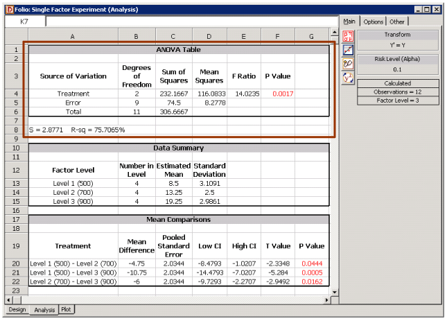
Assuming that the desired significance level is 0.1, since [math]\displaystyle{ p }[/math] value < 0.1, [math]\displaystyle{ {{H}_{0}} }[/math] is rejected and it is concluded that change in the lathe speed has a significant effect on the surface finish. DOE++ displays these results in the ANOVA table, as shown in Figure SingleFactAnalysisSshot1. The values of S and R-sq are the standard error and the coefficient of determination for the model, respectively. These values are explained in Chapter 5 and indicate how well the model fits the data. The values in Figure SingleFactAnalysisSshot1 indicate that the fit of the ANOVA model is fair.
- Figure 6.2: ANOVA table for the data in Table 6.1.
Confidence Interval on the [math]\displaystyle{ i }[/math] th Treatment Mean
The response at each treatment of a single factor experiment can be assumed to be a normal population with a mean of [math]\displaystyle{ {{\mu }_{i}} }[/math] and variance of [math]\displaystyle{ {{\sigma }^{2}} }[/math] provided that the error terms can be assumed to be normally distributed. A point estimator of [math]\displaystyle{ {{\mu }_{i}} }[/math] is the average response at each treatment, [math]\displaystyle{ {{\bar{y}}_{i\cdot }} }[/math] . Since this is a sample average, the associated variance is [math]\displaystyle{ {{\sigma }^{2}}/{{m}_{i}} }[/math] , where [math]\displaystyle{ {{m}_{i}} }[/math] is the number of replicates at the [math]\displaystyle{ i }[/math] th treatment. Therefore, the confidence interval on [math]\displaystyle{ {{\mu }_{i}} }[/math] is based on the [math]\displaystyle{ t }[/math] distribution. Recall from Chapter 3 (inference on population mean when variance is unknown) that:
- [math]\displaystyle{ \begin{align} & {{T}_{0}}= & \frac{{{{\bar{y}}}_{i\cdot }}-{{\mu }_{i}}}{\sqrt{{{{\hat{\sigma }}}^{2}}/{{m}_{i}}}} \\ & = & \frac{{{{\bar{y}}}_{i\cdot }}-{{\mu }_{i}}}{\sqrt{M{{S}_{E}}/{{m}_{i}}}} \end{align} }[/math]
has a [math]\displaystyle{ t }[/math] distribution with degrees of freedom [math]\displaystyle{ =dof(S{{S}_{E}}) }[/math] . Therefore, a 100( [math]\displaystyle{ 1-\alpha }[/math] ) percent confidence interval on the [math]\displaystyle{ i }[/math] th treatment mean, [math]\displaystyle{ {{\mu }_{i}} }[/math] , is:
- [math]\displaystyle{ {{\bar{y}}_{i\cdot }}\pm {{t}_{\alpha /2,dof(S{{S}_{E}})}}\sqrt{\frac{M{{S}_{E}}}{{{m}_{i}}}} }[/math]
For example, for the first treatment of the lathe speed we have:
- [math]\displaystyle{ \begin{align} & {{{\hat{\mu }}}_{1}}= & {{{\bar{y}}}_{1\cdot }} \\ & = & \frac{6+13+7+8}{4} \\ & = & 8.5 \end{align} }[/math]
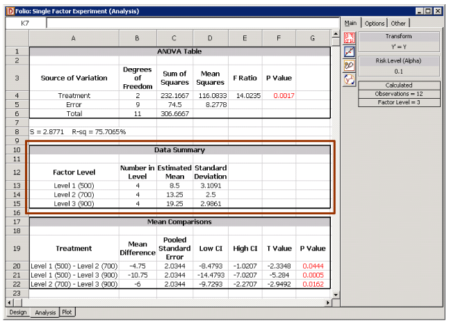
In DOE++, this value is displayed as the Estimated Mean for the first level, as shown in the Data Summary Table in Figure SingleFactAnalysisSshot2. The value displayed as the standard deviation for this level is simply the sample standard deviation calculated using the observations corresponding to this level. The 90% confidence interval for this treatment is:
- [math]\displaystyle{ \begin{align} & = & {{{\bar{y}}}_{1\cdot }}\pm {{t}_{\alpha /2,dof(S{{S}_{E}})}}\sqrt{\frac{M{{S}_{E}}}{{{m}_{i}}}} \\ & = & {{{\bar{y}}}_{1\cdot }}\pm {{t}_{0.05,9}}\sqrt{\frac{M{{S}_{E}}}{4}} \\ & = & 8.5\pm 1.833\sqrt{\frac{(74.5/9)}{4}} \\ & = & 8.5\pm 1.833(1.44) \\ & = & 8.5\pm 2.64 \end{align} }[/math]
The 90% limits on [math]\displaystyle{ {{\mu }_{1}} }[/math] are 5.9 and 11.1, respectively.
- Figure 6.3: Data Summary table for the single factor experiment in Table 6.1.
Confidence Interval on the Difference in Two Treatment Means
The confidence interval on the difference in two treatment means, [math]\displaystyle{ {{\mu }_{i}}-{{\mu }_{j}} }[/math] , is used to compare two levels of the factor at a given significance. If the confidence interval does not include the value of zero, it is concluded that the two levels of the factor are significantly different. The point estimator of [math]\displaystyle{ {{\mu }_{i}}-{{\mu }_{j}} }[/math] is [math]\displaystyle{ {{\bar{y}}_{i\cdot }}-{{\bar{y}}_{j\cdot }} }[/math] . The variance for [math]\displaystyle{ {{\bar{y}}_{i\cdot }}-{{\bar{y}}_{j\cdot }} }[/math] is:
- [math]\displaystyle{ \begin{align} & var({{{\bar{y}}}_{i\cdot }}-{{{\bar{y}}}_{j\cdot }})= & var({{{\bar{y}}}_{i\cdot }})+var({{{\bar{y}}}_{j\cdot }}) \\ & = & {{\sigma }^{2}}/{{m}_{i}}+{{\sigma }^{2}}/{{m}_{j}} \end{align} }[/math]
For balanced designs all [math]\displaystyle{ {{m}_{i}}=m }[/math] . Therefore:
- [math]\displaystyle{ var({{\bar{y}}_{i\cdot }}-{{\bar{y}}_{j\cdot }})=2{{\sigma }^{2}}/m }[/math]
The standard deviation for [math]\displaystyle{ {{\bar{y}}_{i\cdot }}-{{\bar{y}}_{j\cdot }} }[/math] can be obtained by taking the square root of [math]\displaystyle{ var({{\bar{y}}_{i\cdot }}-{{\bar{y}}_{j\cdot }}) }[/math] and is referred to as the pooled standard error:
- [math]\displaystyle{ \begin{align} & Pooled\text{ }Std.\text{ }Error= & \sqrt{var({{{\bar{y}}}_{i\cdot }}-{{{\bar{y}}}_{j\cdot }})} \\ & = & \sqrt{2{{{\hat{\sigma }}}^{2}}/m} \end{align} }[/math]
The [math]\displaystyle{ t }[/math] statistic for the difference is:
- [math]\displaystyle{ \begin{align} & {{T}_{0}}= & \frac{{{{\bar{y}}}_{i\cdot }}-{{{\bar{y}}}_{j\cdot }}-({{\mu }_{i}}-{{\mu }_{j}})}{\sqrt{2{{{\hat{\sigma }}}^{2}}/m}} \\ & = & \frac{{{{\bar{y}}}_{i\cdot }}-{{{\bar{y}}}_{j\cdot }}-({{\mu }_{i}}-{{\mu }_{j}})}{\sqrt{2M{{S}_{E}}/m}} \end{align} }[/math]
Then a 100(1- [math]\displaystyle{ \alpha }[/math] ) percent confidence interval on the difference in two treatment means, [math]\displaystyle{ {{\mu }_{i}}-{{\mu }_{j}} }[/math] , is:
- [math]\displaystyle{ {{\bar{y}}_{i\cdot }}-{{\bar{y}}_{j\cdot }}\pm {{t}_{\alpha /2,dof(S{{S}_{E}})}}\sqrt{\frac{2M{{S}_{E}}}{m}} }[/math]
For example, an estimate of the difference in the first and second treatment means of the lathe speed, [math]\displaystyle{ {{\mu }_{1}}-{{\mu }_{2}} }[/math] , is:
- [math]\displaystyle{ \begin{align} & {{{\hat{\mu }}}_{1}}-{{{\hat{\mu }}}_{2}}= & {{{\bar{y}}}_{1\cdot }}-{{{\bar{y}}}_{2\cdot }} \\ & = & 8.5-13.25 \\ & = & -4.75 \end{align} }[/math]
The pooled standard error for this difference is:
- [math]\displaystyle{ \begin{align} & Pooled\text{ }Std.\text{ }Error= & \sqrt{var({{{\bar{y}}}_{1\cdot }}-{{{\bar{y}}}_{2\cdot }})} \\ & = & \sqrt{2{{{\hat{\sigma }}}^{2}}/m} \\ & = & \sqrt{2M{{S}_{E}}/m} \\ & = & \sqrt{\frac{2(74.5/9)}{4}} \\ & = & 2.0344 \end{align} }[/math]
To test [math]\displaystyle{ {{H}_{0}}\ \ :\ \ {{\mu }_{1}}-{{\mu }_{2}}=0 }[/math] , the [math]\displaystyle{ t }[/math] statistic is:
- [math]\displaystyle{ \begin{align} & {{t}_{0}}= & \frac{{{{\bar{y}}}_{1\cdot }}-{{{\bar{y}}}_{2\cdot }}-({{\mu }_{1}}-{{\mu }_{2}})}{\sqrt{2M{{S}_{E}}/m}} \\ & = & \frac{-4.75-(0)}{\sqrt{\tfrac{2(74.5/9)}{4}}} \\ & = & \frac{-4.75}{2.0344} \\ & = & -2.3348 \end{align} }[/math]
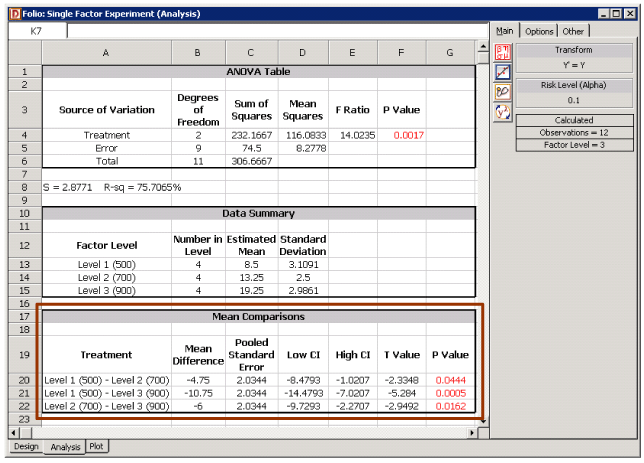
In DOE++, the value of the statistic is displayed in the Mean Comparisons table under the column T Value as shown in Figure SingleFactAnalysisSshot3. The 90% confidence interval on the difference [math]\displaystyle{ {{\mu }_{1}}-{{\mu }_{2}} }[/math] is:
- [math]\displaystyle{ \begin{align} & = & {{{\bar{y}}}_{1\cdot }}-{{{\bar{y}}}_{2\cdot }}\pm {{t}_{\alpha /2,dof(S{{S}_{E}})}}\sqrt{\frac{2M{{S}_{E}}}{m}} \\ & = & {{{\bar{y}}}_{1\cdot }}-{{{\bar{y}}}_{2\cdot }}\pm {{t}_{0.05,9}}\sqrt{\frac{2M{{S}_{E}}}{m}} \\ & = & -4.75\pm 1.833\sqrt{\frac{2(74.5/9)}{4}} \\ & = & -4.75\pm 1.833(2.0344) \\ & = & -4.75\pm 3.729 \end{align} }[/math]
Hence the 90% limits on [math]\displaystyle{ {{\mu }_{1}}-{{\mu }_{2}} }[/math] are [math]\displaystyle{ -8.479 }[/math] and [math]\displaystyle{ -1.021 }[/math] , respectively. These values are displayed under the Low CI and High CI columns in Figure SingleFactAnalysisSshot3. Since the confidence interval for this pair of means does not included zero, it can be concluded that these means are significantly different at 90% confidence. This conclusion can also be arrived at using the [math]\displaystyle{ p }[/math] value noting that the hypothesis is two-sided. The [math]\displaystyle{ p }[/math] value corresponding to the statistic [math]\displaystyle{ {{t}_{0}}=-2.3348 }[/math] , based on the [math]\displaystyle{ t }[/math] distribution with 9 degrees of freedom is:
- [math]\displaystyle{ \begin{align} & p\text{ }value= & 2\times (1-P(T\le |{{t}_{0}}|)) \\ & = & 2\times (1-P(T\le 2.3348)) \\ & = & 2\times (1-0.9778) \\ & = & 0.0444 \end{align} }[/math]
Since [math]\displaystyle{ p }[/math] value < 0.1, the means are significantly different at 90% confidence. Bounds on the difference between other treatment pairs can be obtained in a similar manner and it is concluded that all treatments are significantly different.
Residual Analysis
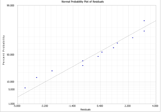
Plots of residuals, [math]\displaystyle{ {{e}_{ij}} }[/math] , similar to the ones discussed in the previous chapters on regression, are used to ensure that the assumptions associated with the ANOVA model are not violated. The ANOVA model assumes that the random error terms, [math]\displaystyle{ {{\epsilon }_{ij}} }[/math] , are normally and independently distributed with the same variance for each treatment. The normality assumption can be checked by obtaining a normal probability plot of the residuals.
- Figure 6.4.png|center]]
- Figure 6.4: Mean Comparisons table for the data in Table 6.1.
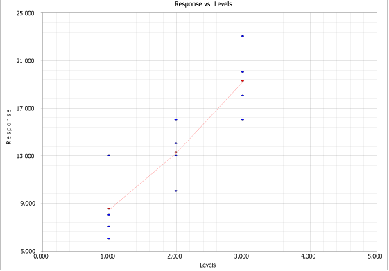
Equality of variance is checked by plotting residuals against the treatments and the treatment averages, [math]\displaystyle{ {{\bar{y}}_{i\cdot }} }[/math] (also referred to as fitted values), and inspecting the spread in the residuals. If a pattern is seen in these plots, then this indicates the need to use a suitable transformation on the response that will ensure variance equality. Box-Cox transformations are discussed in the next section. To check for independence of the random error terms residuals are plotted against time or run-order to ensure that a pattern does not exist in these plots. Residual plots for the given example are shown in Figures SingleFactExResidualPlots1 and SingleFactExResidualPlots2. The plots show that the assumptions associated with the ANOVA model are not violated.
- Figure 6.5: Normal probability plot of residuals for the single factor experiment in Table 6.1.
- Figure 6.6: Plot of residuals against fitted values for the single factor experiment in Table 6.1.
Box-Cox Method
Transformations on the response may be used when residual plots for an experiment show a pattern. This indicates that the equality of variance does not hold for the residuals of the given model. The Box-Cox method can be used to automatically identify a suitable power transformation for the data based on the relation:
- [math]\displaystyle{ {{Y}^{*}}={{Y}^{\lambda }} }[/math]
[math]\displaystyle{ \lambda }[/math] is determined using the given data such that [math]\displaystyle{ S{{S}_{E}} }[/math] is minimized. The values of [math]\displaystyle{ {{Y}^{\lambda }} }[/math] are not used as is because of issues related to calculation or comparison of [math]\displaystyle{ S{{S}_{E}} }[/math] values for different values of [math]\displaystyle{ \lambda }[/math] . For example, for [math]\displaystyle{ \lambda =0 }[/math] all response values will become 1. Therefore, the following relation is used to obtain [math]\displaystyle{ {{Y}^{\lambda }} }[/math] :
- [math]\displaystyle{ {{Y}^{\lambda }}=\{\begin{matrix} \frac{{{Y}^{\lambda }}-1}{\lambda {{{\dot{y}}}^{\lambda -1}}} \\ \dot{y}\ln y \\ \end{matrix}\text{ }\begin{matrix} \lambda \ne 0\begin{matrix} \\ \\ \end{matrix} \\ \lambda =0 \\ \end{matrix} }[/math]
where [math]\displaystyle{ \dot{y}={{\ln }^{-1}}[(1/n)\mathop{}_{}^{}\ln y] }[/math] .
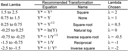
Once all [math]\displaystyle{ {{Y}^{\lambda }} }[/math] values are obtained for a value of [math]\displaystyle{ \lambda }[/math] , the corresponding [math]\displaystyle{ S{{S}_{E}} }[/math] for these values is obtained using [math]\displaystyle{ {{y}^{\lambda \prime }}[I-H]{{y}^{\lambda }} }[/math] . The process is repeated for a number of [math]\displaystyle{ \lambda }[/math] values to obtain a plot of [math]\displaystyle{ S{{S}_{E}} }[/math] against [math]\displaystyle{ \lambda }[/math] . Then the value of [math]\displaystyle{ \lambda }[/math] corresponding to the minimum [math]\displaystyle{ S{{S}_{E}} }[/math] is selected as the required transformation for the given data. DOE++ plots [math]\displaystyle{ \ln S{{S}_{E}} }[/math] values against [math]\displaystyle{ \lambda }[/math] values because the range of [math]\displaystyle{ S{{S}_{E}} }[/math] values is large and if this is not done, all values cannot be displayed on the same plot. The range of search for the best [math]\displaystyle{ \lambda }[/math] value in the software is from [math]\displaystyle{ -5 }[/math] to [math]\displaystyle{ 5 }[/math] , because larger values of of [math]\displaystyle{ \lambda }[/math] are usually not meaningful. DOE++ also displays a recommended transformation based on the best [math]\displaystyle{ \lambda }[/math] value obtained as per Table 6.2.
- Figure 6.2: Recommended Box-Cox power transformations.
Confidence intervals on the selected [math]\displaystyle{ \lambda }[/math] values are also available. Let [math]\displaystyle{ S{{S}_{E}}(\lambda ) }[/math] be the value of [math]\displaystyle{ S{{S}_{E}} }[/math] corresponding to the selected value of [math]\displaystyle{ \lambda }[/math] . Then, to calculate the 100(1- [math]\displaystyle{ \alpha }[/math] ) percent confidence intervals on [math]\displaystyle{ \lambda }[/math] , we need to calculate [math]\displaystyle{ S{{S}^{*}} }[/math] as shown next:
- [math]\displaystyle{ S{{S}^{*}}=S{{S}_{E}}(\lambda )\left( 1+\frac{t_{\alpha /2,dof(S{{S}_{E}})}^{2}}{dof(S{{S}_{E}})} \right) }[/math]
The required limits for [math]\displaystyle{ \lambda }[/math] are the two values of [math]\displaystyle{ \lambda }[/math] corresponding to the value [math]\displaystyle{ S{{S}^{*}} }[/math] (on the plot of [math]\displaystyle{ S{{S}_{E}} }[/math] against [math]\displaystyle{ \lambda }[/math] ). If the limits for [math]\displaystyle{ \lambda }[/math] do not include the value of one, then the transformation is applicable for the given data.
Note that the power transformations are not defined for response values that are negative or zero. DOE++ deals with negative and zero response values using the following equations (that involve addition of a suitable quantity to all of the response values if a zero or negative response value is encountered).
- [math]\displaystyle{ \begin{align} & y(i)= & y(i)+\left| {{y}_{\min }} \right|\times 1.1\text{ Negative Response} \\ & y(i)= & y(i)+1\text{ Zero Response} \end{align} }[/math]
Here [math]\displaystyle{ {{y}_{\min }} }[/math] represents the minimum response value and [math]\displaystyle{ \left| {{y}_{\min }} \right| }[/math] represents the absolute value of the minimum response.
Example 1
To illustrate the Box-Cox method, consider the experiment given in Table 6.1. Eqn. (BoxCoxEquation) can be used to calculate transformed response values for various values of [math]\displaystyle{ \lambda }[/math] . Knowing the hat matrix, [math]\displaystyle{ H }[/math] , [math]\displaystyle{ S{{S}_{E}} }[/math] values corresponding to each of these [math]\displaystyle{ \lambda }[/math] values can easily be obtained using [math]\displaystyle{ {{y}^{\lambda \prime }}[I-H]{{y}^{\lambda }} }[/math] . [math]\displaystyle{ S{{S}_{E}} }[/math] values calculated for [math]\displaystyle{ \lambda }[/math] values between [math]\displaystyle{ -5 }[/math] and [math]\displaystyle{ 5 }[/math] for the given data are shown below:
- [math]\displaystyle{ \begin{matrix} \lambda & {} & S{{S}_{E}} & \ln S{{S}_{E}} \\ {} & {} & {} & {} \\ -5 & {} & 5947.8 & 8.6908 \\ -4 & {} & 1946.4 & 7.5737 \\ -3 & {} & 696.5 & 6.5461 \\ -2 & {} & 282.2 & 5.6425 \\ -1 & {} & 135.8 & 4.9114 \\ 0 & {} & 83.9 & 4.4299 \\ 1 & {} & 74.5 & 4.3108 \\ 2 & {} & 101.0 & 4.6154 \\ 3 & {} & 190.4 & 5.2491 \\ 4 & {} & 429.5 & 6.0627 \\ 5 & {} & 1057.6 & -6.9638 \\ \end{matrix} }[/math]
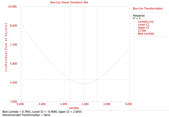
A plot of [math]\displaystyle{ \ln S{{S}_{E}} }[/math] for various [math]\displaystyle{ \lambda }[/math] values, as obtained from DOE++, is shown in Figure BoxCoxPlot. The value of [math]\displaystyle{ \lambda }[/math] that gives the minimum [math]\displaystyle{ S{{S}_{E}} }[/math] is identified as 0.7841. The [math]\displaystyle{ S{{S}_{E}} }[/math] value corresponding to this value of [math]\displaystyle{ \lambda }[/math] is 73.74. A 90% confidence interval on this [math]\displaystyle{ \lambda }[/math] value is calculated as follows. Using Eqn. (BoxCoxCI), [math]\displaystyle{ S{{S}^{*}} }[/math] can be obtained:
- [math]\displaystyle{ \begin{align} & S{{S}^{*}}= & S{{S}_{E}}(\lambda )\left( 1+\frac{t_{\alpha /2,dof(S{{S}_{E}})}^{2}}{dof(S{{S}_{E}})} \right) \\ & = & 73.74\left( 1+\frac{t_{0.05,9}^{2}}{9} \right) \\ & = & 73.74\left( 1+\frac{{{1.833}^{2}}}{9} \right) \\ & = & 101.27 \end{align} }[/math]
Therefore, [math]\displaystyle{ \ln S{{S}^{*}}=4.6178 }[/math] . The [math]\displaystyle{ \lambda }[/math] values corresponding to this value from Figure BoxCoxPlot are [math]\displaystyle{ -0.4686 }[/math] and [math]\displaystyle{ 2.0052 }[/math] . Therefore, the 90% confidence limits on are [math]\displaystyle{ -0.4689 }[/math] and [math]\displaystyle{ 2.0055 }[/math] . Since the confidence limits include the value of 1, this indicates that a transformation is not required for the data in Table 6.1.
- Figure 6.7: Box-Cox power transformation plot for the data in Table 6.1.
Experiments with Several Factors - Factorial Experiments
Experiments with two or more factors are encountered frequently. The best way to carry out such experiments is by using factorial experiments. Factorial experiments are experiments in which all combinations of factors are investigated in each replicate of the experiment. Factorial experiments are the only means to completely and systematically study interactions between factors in addition to identifying significant factors. One-factor-at-a-time experiments (where each factor is investigated separately by keeping all the remaining factors constant) do not reveal the interaction effects between the factors. Further, in one-factor-at-a-time experiments full randomization is not possible.
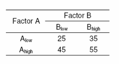
To illustrate factorial experiments consider an experiment where the response is investigated for two factors, [math]\displaystyle{ A }[/math] and [math]\displaystyle{ B }[/math] . Assume that the response is studied at two levels of factor [math]\displaystyle{ A }[/math] with [math]\displaystyle{ {{A}_{\text{low}}} }[/math] representing the lower level of [math]\displaystyle{ A }[/math] and [math]\displaystyle{ {{A}_{\text{high}}} }[/math] representing the higher level of [math]\displaystyle{ A }[/math] . Similarly, let [math]\displaystyle{ {{B}_{\text{low}}} }[/math] and [math]\displaystyle{ {{B}_{\text{high}}} }[/math] represent the two levels of factor [math]\displaystyle{ B }[/math] that are being investigated in this experiment. Since there are two factors with two levels, a total of [math]\displaystyle{ 2\times 2=4 }[/math] combinations exist ( [math]\displaystyle{ {{A}_{\text{low}}} }[/math] - [math]\displaystyle{ {{B}_{\text{low}}} }[/math] , - [math]\displaystyle{ {{B}_{\text{high}}} }[/math] , [math]\displaystyle{ {{A}_{\text{high}}} }[/math] - [math]\displaystyle{ {{B}_{\text{low}}} }[/math] , - [math]\displaystyle{ {{B}_{\text{high}}} }[/math] ). Thus, four runs are required for each replicate if a factorial experiment is to be carried out in this case. Assume that the response values for each of these four possible combinations are obtained as shown in Table 6.3.
- Table 6.3: Two-factor factorial experiment.
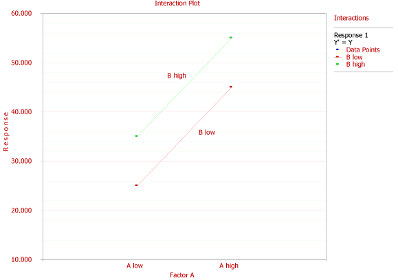
- Figure 6.8: Interaction plot for the data in Table 6.3.
Investigating Factor Effects
The effect of factor [math]\displaystyle{ A }[/math] on the response can be obtained by taking the difference between the average response when [math]\displaystyle{ A }[/math] is high and the average response when [math]\displaystyle{ A }[/math] is low. The change in the response due to a change in the level of a factor is called the main effect of the factor. The main effect of [math]\displaystyle{ A }[/math] as per the response values in Table 6.3 is:
- [math]\displaystyle{ \begin{align} & A= & Average\text{ }response\text{ }at\text{ }{{A}_{\text{high}}}-Average\text{ }response\text{ }at\text{ }{{A}_{\text{low}}} \\ & = & \frac{45+55}{2}-\frac{25+35}{2} \\ & = & 50-30 \\ & = & 20 \end{align} }[/math]
Therefore, when [math]\displaystyle{ A }[/math] is changed from the lower level to the higher level, the response increases by 20 units. A plot of the response for the two levels of [math]\displaystyle{ A }[/math] at different levels of [math]\displaystyle{ B }[/math] is shown in Figure interaction1. The plot shows that change in the level of [math]\displaystyle{ A }[/math] leads to an increase in the response by 20 units regardless of the level of [math]\displaystyle{ B }[/math] . Therefore, no interaction exists in this case as indicated by the parallel lines on the plot. The main effect of [math]\displaystyle{ B }[/math] can be obtained as:
- [math]\displaystyle{ \begin{align} & B= & Average\text{ }response\text{ }at\text{ }{{B}_{\text{high}}}-Average\text{ }response\text{ }at\text{ }{{B}_{\text{low}}} \\ & = & \frac{35+55}{2}-\frac{25+45}{2} \\ & = & 45-35 \\ & = & 10 \end{align} }[/math]
Investigating Interactions
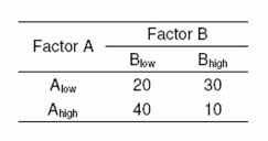
Now assume that the response values for each of the four treatment combinations were obtained as shown in Table 6.4. The main effect of [math]\displaystyle{ A }[/math] in this case is:
- [math]\displaystyle{ \begin{align} & A= & Average\text{ }response\text{ }at\text{ }{{A}_{\text{high}}}-Average\text{ }response\text{ }at\text{ }{{A}_{\text{low}}} \\ & = & \frac{40+10}{2}-\frac{20+30}{2} \\ & = & 0 \end{align} }[/math]
- Figure 6.4: Two-factor factorial experiment.
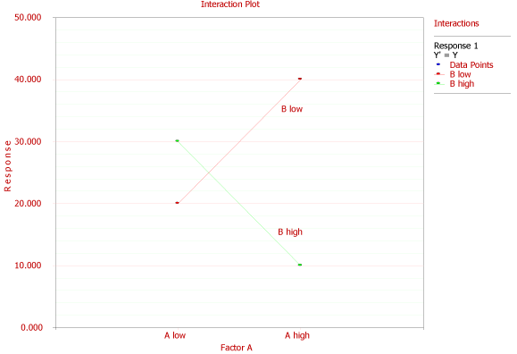
It appears that [math]\displaystyle{ A }[/math] does not have an effect on the response. However, a plot of the response of [math]\displaystyle{ A }[/math] at different levels of [math]\displaystyle{ B }[/math] shows that the response does change with the levels of [math]\displaystyle{ A }[/math] but the effect of [math]\displaystyle{ A }[/math] on the response is dependent on the level of [math]\displaystyle{ B }[/math] (see Figure interaction2). Therefore, an interaction between [math]\displaystyle{ A }[/math] and [math]\displaystyle{ B }[/math] exists in this case (as indicated by the non-parallel lines of the figure). The interaction effect between [math]\displaystyle{ A }[/math] and [math]\displaystyle{ B }[/math] can be calculated as follows:
- Figure 6.9: Interaction plot for the data in Table 6.4.
- [math]\displaystyle{ \begin{align} & AB= & Average\text{ }response\text{ }at\text{ }{{A}_{\text{high}}}\text{-}{{B}_{\text{high}}}\text{ }and\text{ }{{A}_{\text{low}}}\text{-}{{B}_{\text{low}}}- \\ & & Average\text{ }response\text{ }at\text{ }{{A}_{\text{low}}}\text{-}{{B}_{\text{high}}}\text{ }and\text{ }{{A}_{\text{high}}}\text{-}{{B}_{\text{low}}} \\ & = & \frac{10+20}{2}-\frac{40+30}{2} \\ & = & -20 \end{align} }[/math]
Note that in this case, if a one-factor-at-a-time experiment were used to investigate the effect of factor [math]\displaystyle{ A }[/math] on the response, it would lead to incorrect conclusions. For example, if the response at factor [math]\displaystyle{ A }[/math] was studied by holding [math]\displaystyle{ B }[/math] constant at its lower level, then the main effect of [math]\displaystyle{ A }[/math] would be obtained as [math]\displaystyle{ 40-20=20 }[/math] , indicating that the response increases by 20 units when the level of [math]\displaystyle{ A }[/math] is changed from low to high. On the other hand, if the response at factor [math]\displaystyle{ A }[/math] was studied by holding [math]\displaystyle{ B }[/math] constant at its higher level then the main effect of [math]\displaystyle{ A }[/math] would be obtained as [math]\displaystyle{ 10-30=-20 }[/math] , indicating that the response decreases by 20 units when the level of [math]\displaystyle{ A }[/math] is changed from low to high.
Analysis of General Factorial Experiments
In DOE++, factorial experiments are referred to as factorial designs. The experiments explained in this section are referred to as general factorial designs. This is done to distinguish these experiments from the other factorial designs supported by DOE++ (see Figure FactorialDesignsSshot). The other designs (such as the 2 level full factorial designs that are explained in Chapter 7) are special cases of these experiments in which factors are limited to a specified number of levels. The ANOVA model for the analysis of factorial experiments is formulated as shown next. Assume a factorial experiment in which the effect of two factors, [math]\displaystyle{ A }[/math] and [math]\displaystyle{ B }[/math] , on the response is being investigated. Let there be [math]\displaystyle{ {{n}_{a}} }[/math] levels of factor [math]\displaystyle{ A }[/math] and [math]\displaystyle{ {{n}_{b}} }[/math] levels of factor [math]\displaystyle{ B }[/math] . The ANOVA model for this experiment can be stated as:
- [math]\displaystyle{ {{Y}_{ijk}}=\mu +{{\tau }_{i}}+{{\delta }_{j}}+{{(\tau \delta )}_{ij}}+{{\epsilon }_{ijk}} }[/math]
where:
• [math]\displaystyle{ \mu }[/math] represents the overall mean effect
• [math]\displaystyle{ {{\tau }_{i}} }[/math] is the effect of the [math]\displaystyle{ i }[/math] th level of factor [math]\displaystyle{ A }[/math] ( [math]\displaystyle{ i=1,2,...,{{n}_{a}} }[/math] )
• [math]\displaystyle{ {{\delta }_{j}} }[/math] is the effect of the [math]\displaystyle{ j }[/math] th level of factor [math]\displaystyle{ B }[/math] ( [math]\displaystyle{ j=1,2,...,{{n}_{b}} }[/math] )
• [math]\displaystyle{ {{(\tau \delta )}_{ij}} }[/math] represents the interaction effect between [math]\displaystyle{ A }[/math] and [math]\displaystyle{ B }[/math]
• [math]\displaystyle{ {{\epsilon }_{ijk}} }[/math] represents the random error terms (which are assumed to be normally distributed with a mean of zero and variance of [math]\displaystyle{ {{\sigma }^{2}} }[/math] )
• and the subscript [math]\displaystyle{ k }[/math] denotes the [math]\displaystyle{ m }[/math] replicates ( [math]\displaystyle{ k=1,2,...,m }[/math] )
Since the effects [math]\displaystyle{ {{\tau }_{i}} }[/math] , [math]\displaystyle{ {{\delta }_{j}} }[/math] and [math]\displaystyle{ {{(\tau \delta )}_{ij}} }[/math] represent deviations from the overall mean, the following constraints exist:
- [math]\displaystyle{ \underset{i=1}{\overset{{{n}_{a}}}{\mathop \sum }}\,{{\tau }_{i}}=0 }[/math]
- Figure 6.10: Factorial experiments availiable in DOE++.
[math]\displaystyle{ \begin{align} & \underset{j=1}{\overset{{{n}_{b}}}{\mathop \sum }}\,{{\delta }_{j}}= & 0 \\ & \underset{i=1}{\overset{{{n}_{a}}}{\mathop \sum }}\,{{(\tau \delta )}_{ij}}= & 0 \\ & \underset{j=1}{\overset{{{n}_{b}}}{\mathop \sum }}\,{{(\tau \delta )}_{ij}}= & 0 \end{align} }[/math]
Hypothesis Tests in General Factorial Experiments
These tests are used to check whether each of the factors investigated in the experiment is significant or not. For the previous example, with two factors, [math]\displaystyle{ A }[/math] and [math]\displaystyle{ B }[/math] , and their interaction, [math]\displaystyle{ AB }[/math] , the statements for the hypothesis tests can be formulated as follows:
- [math]\displaystyle{ \begin{align} & \begin{matrix} 1. & {} \\ \end{matrix}{{H}_{0}}: & {{\tau }_{1}}={{\tau }_{2}}=...={{\tau }_{{{n}_{a}}}}=0\text{ (Main effect of }A\text{ is absent)} \\ & \begin{matrix} {} & {} \\ \end{matrix}{{H}_{1}}: & {{\tau }_{i}}\ne 0\text{ for at least one }i \\ & \begin{matrix} 2. & {} \\ \end{matrix}{{H}_{0}}: & {{\delta }_{1}}={{\delta }_{2}}=...={{\delta }_{{{n}_{b}}}}=0\text{ (Main effect of }B\text{ is absent)} \\ & \begin{matrix} {} & {} \\ \end{matrix}{{H}_{1}}: & {{\delta }_{j}}\ne 0\text{ for at least one }j \\ & \begin{matrix} 3. & {} \\ \end{matrix}{{H}_{0}}: & {{(\tau \delta )}_{11}}={{(\tau \delta )}_{12}}=...={{(\tau \delta )}_{{{n}_{a}}{{n}_{b}}}}=0\text{ (Interaction }AB\text{ is absent)} \\ & \begin{matrix} {} & {} \\ \end{matrix}{{H}_{1}}: & {{(\tau \delta )}_{ij}}\ne 0\text{ for at least one }ij \end{align} }[/math]
The test statistics for the three tests are as follows:
- [math]\displaystyle{ \begin{align} & & \begin{matrix} 1. & {{({{F}_{0}})}_{A}}=\frac{M{{S}_{A}}}{M{{S}_{E}}}\text{ } \\ \end{matrix} \\ & & \text{ where }M{{S}_{A}}\text{ is the mean square due to factor }A\text{ and} \\ & & \text{ }M{{S}_{E}}\text{ is the error mean square} \\ & & \begin{matrix} 2. & {{({{F}_{0}})}_{B}}=\frac{M{{S}_{B}}}{M{{S}_{E}}}\text{ } \\ \end{matrix} \\ & & \text{ where }M{{S}_{B}}\text{ is the mean square due to factor }B\text{ and} \\ & & \text{ }M{{S}_{E}}\text{ is the error mean square} \\ & & \begin{matrix} 3. & {{({{F}_{0}})}_{AB}}=\frac{M{{S}_{AB}}}{M{{S}_{E}}}\text{ } \\ \end{matrix} \\ & & \text{ where }M{{S}_{AB}}\text{ is the mean square due to interaction }AB\text{ and} \\ & & \text{ }M{{S}_{E}}\text{ is the error mean square} \end{align} }[/math]
The tests are identical to the partial [math]\displaystyle{ F }[/math] test explained in Chapter 5. The sum of squares for these tests (to obtain the mean squares) are calculated by splitting the model sum of squares into the extra sum of squares due to each factor. The extra sum of squares calculated for each of the factors may either be partial or sequential. For the present example, if the extra sum of squares used is sequential, then the model sum of squares can be written as:
- [math]\displaystyle{ S{{S}_{TR}}=S{{S}_{A}}+S{{S}_{B}}+S{{S}_{AB}} }[/math]
where [math]\displaystyle{ S{{S}_{TR}} }[/math] represents the model sum of squares, [math]\displaystyle{ S{{S}_{A}} }[/math] represents the sequential sum of squares due to factor [math]\displaystyle{ A }[/math] , [math]\displaystyle{ S{{S}_{B}} }[/math] represents the sequential sum of squares due to factor and [math]\displaystyle{ S{{S}_{AB}} }[/math] represents the sequential sum of squares due to the interaction [math]\displaystyle{ AB }[/math] .
The mean squares are obtained by dividing the sum of squares by the associated degrees of freedom. Once the mean squares are known the test statistics can be calculated. For example, the test statistic to test the significance of factor [math]\displaystyle{ A }[/math] (or the hypothesis [math]\displaystyle{ {{H}_{0}}\ \ :\ \ {{\tau }_{i}}=0 }[/math] ) can then be obtained as:
- [math]\displaystyle{ \begin{align} & {{({{F}_{0}})}_{A}}= & \frac{M{{S}_{A}}}{M{{S}_{E}}} \\ & = & \frac{S{{S}_{A}}/dof(S{{S}_{A}})}{S{{S}_{E}}/dof(S{{S}_{E}})} \end{align} }[/math]
Similarly the test statistic to test significance of factor [math]\displaystyle{ B }[/math] and the interaction [math]\displaystyle{ AB }[/math] can be respectively obtained as:
- [math]\displaystyle{ \begin{align} & {{({{F}_{0}})}_{B}}= & \frac{M{{S}_{B}}}{M{{S}_{E}}} \\ & = & \frac{S{{S}_{B}}/dof(S{{S}_{B}})}{S{{S}_{E}}/dof(S{{S}_{E}})} \\ & {{({{F}_{0}})}_{AB}}= & \frac{M{{S}_{AB}}}{M{{S}_{E}}} \\ & = & \frac{S{{S}_{AB}}/dof(S{{S}_{AB}})}{S{{S}_{E}}/dof(S{{S}_{E}})} \end{align} }[/math]
It is recommended to conduct the test for interactions before conducting the test for the main effects. This is because, if an interaction is present, then the main effect of the factor depends on the level of the other factors and looking at the main effect is of little value. However, if the interaction is absent then the main effects become important.
Example 2
Consider an experiment to investigate the effect of speed and type of fuel additive used on the mileage of a sports utility vehicle. Three speeds and two types of fuel additives are investigated. Each of the treatment combinations are replicated three times. The mileage values observed are displayed in Table 6.5.
- Figure 6.5: Mileage data for different speeds and fuel additive types.
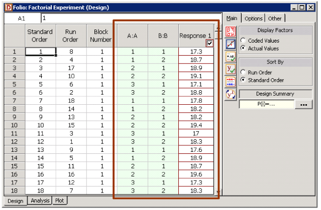
The experimental design for the data in Table 6.5 is shown in Figure FactDesingSshot. In the figure, the factor Speed is represented as factor [math]\displaystyle{ A }[/math] and the factor Fuel Additive is represented as factor [math]\displaystyle{ B }[/math] . The experimenter would like to investigate if speed, fuel additive or the interaction between speed and fuel additive affects the mileage of the sports utility vehicle. In other words, the following hypotheses need to be tested:
[math]\displaystyle{ \begin{align}
& \begin{matrix}
1. & {} \\
\end{matrix}{{H}_{0}}: & {{\tau }_{1}}={{\tau }_{2}}={{\tau }_{3}}=0\text{ (No main effect of factor }A\text{, speed)} \\
& \begin{matrix}
{} & {} \\
\end{matrix}{{H}_{1}}: & {{\tau }_{i}}\ne 0\text{ for at least one }i \\
& \begin{matrix}
2. & {} \\
\end{matrix}{{H}_{0}}: & {{\delta }_{1}}={{\delta }_{2}}={{\delta }_{3}}=0\text{ (No main effect of factor }B\text{, fuel additive)} \\
& \begin{matrix}
{} & {} \\
\end{matrix}{{H}_{1}}: & {{\delta }_{j}}\ne 0\text{ for at least one }j \\
& \begin{matrix}
3. & {} \\
\end{matrix}{{H}_{0}}: & {{(\tau \delta )}_{11}}={{(\tau \delta )}_{12}}=...={{(\tau \delta )}_{33}}=0\text{ (No interaction }AB\text{)} \\
& \begin{matrix}
{} & {} \\
\end{matrix}{{H}_{1}}: & {{(\tau \delta )}_{ij}}\ne 0\text{ for at least one }ij
\end{align} }[/math]
The test statistics for the three tests are:
- [math]\displaystyle{ \begin{align} & & \begin{matrix} 1. & {{({{F}_{0}})}_{A}}=\frac{M{{S}_{A}}}{M{{S}_{E}}}\text{ } \\ \end{matrix} \\ & & \text{ where }M{{S}_{A}}\text{ is the mean square for factor }A\text{ and} \\ & & \text{ }M{{S}_{E}}\text{ is the error mean square} \\ & & \begin{matrix} 2. & {{({{F}_{0}})}_{B}}=\frac{M{{S}_{B}}}{M{{S}_{E}}}\text{ } \\ \end{matrix} \\ & & \text{ where }M{{S}_{B}}\text{ is the mean square for factor }B\text{ and} \\ & & \text{ }M{{S}_{E}}\text{ is the error mean square} \\ & & \begin{matrix} 3. & {{({{F}_{0}})}_{AB}}=\frac{M{{S}_{AB}}}{M{{S}_{E}}}\text{ } \\ \end{matrix} \\ & & \text{ where }M{{S}_{AB}}\text{ is the mean square for interaction }AB\text{ and} \\ & & \text{ }M{{S}_{E}}\text{ is the error mean square} \end{align} }[/math]
- Figure 6.11: Experimental design for the data in Table 6.5.
The ANOVA model for this experiment can be written as:
- [math]\displaystyle{ {{Y}_{ijk}}=\mu +{{\tau }_{i}}+{{\delta }_{j}}+{{(\tau \delta )}_{ij}}+{{\epsilon }_{ijk}} }[/math]
where [math]\displaystyle{ {{\tau }_{i}} }[/math] represents the [math]\displaystyle{ i }[/math] th treatment of factor [math]\displaystyle{ A }[/math] (speed) with [math]\displaystyle{ i }[/math] =1, 2, 3; [math]\displaystyle{ {{\delta }_{j}} }[/math] represents the [math]\displaystyle{ j }[/math] th treatment of factor [math]\displaystyle{ B }[/math] (fuel additive) with [math]\displaystyle{ j }[/math] =1, 2; and [math]\displaystyle{ {{(\tau \delta )}_{ij}} }[/math] represents the interaction effect. In order to calculate the test statistics, it is convenient to express the ANOVA model of Eqn. (TwoFactModelEx) in the form [math]\displaystyle{ y=X\beta +\epsilon }[/math] . This can be done as explained next.
Expression of the ANOVA Model as [math]\displaystyle{ y=X\beta +\epsilon }[/math]
Since the effects [math]\displaystyle{ {{\tau }_{i}} }[/math] , [math]\displaystyle{ {{\delta }_{j}} }[/math] and [math]\displaystyle{ {{(\tau \delta )}_{ij}} }[/math] represent deviations from the overall mean, the following constraints exist. Constraints on [math]\displaystyle{ {{\tau }_{i}} }[/math] are:
- [math]\displaystyle{ \begin{align} & \underset{i=1}{\overset{3}{\mathop \sum }}\,{{\tau }_{i}}= & 0 \\ & \text{or }{{\tau }_{1}}+{{\tau }_{2}}+{{\tau }_{3}}= & 0 \end{align} }[/math]
Therefore, only two of the [math]\displaystyle{ {{\tau }_{i}} }[/math] effects are independent. Assuming that [math]\displaystyle{ {{\tau }_{1}} }[/math] and [math]\displaystyle{ {{\tau }_{2}} }[/math] are independent, [math]\displaystyle{ {{\tau }_{3}}=-({{\tau }_{1}}+{{\tau }_{2}}) }[/math] . (The null hypothesis to test the significance of factor [math]\displaystyle{ A }[/math] can be rewritten using only the independent effects as [math]\displaystyle{ {{H}_{0}}\ \ :\ \ {{\tau }_{1}}={{\tau }_{2}}=0 }[/math] .) DOE++ displays only the independent effects because only these effects are important to the analysis. The independent effects, [math]\displaystyle{ {{\tau }_{1}} }[/math] and [math]\displaystyle{ {{\tau }_{2}} }[/math] , are displayed as A[1] and A[2] respectively because these are the effects associated with factor [math]\displaystyle{ A }[/math] (speed).
Constraints on [math]\displaystyle{ {{\delta }_{j}} }[/math] are:
- [math]\displaystyle{ \begin{align} & \underset{j=1}{\overset{2}{\mathop \sum }}\,{{\delta }_{j}}= & 0 \\ & \text{or }{{\delta }_{1}}+{{\delta }_{2}}= & 0 \end{align} }[/math]
Therefore, only one of the [math]\displaystyle{ {{\delta }_{j}} }[/math] effects are independent. Assuming that [math]\displaystyle{ {{\delta }_{1}} }[/math] is independent, [math]\displaystyle{ {{\delta }_{2}}=-{{\delta }_{1}} }[/math] . (The null hypothesis to test the significance of factor [math]\displaystyle{ B }[/math] can be rewritten using only the independent effect as [math]\displaystyle{ {{H}_{0}}\ \ :\ \ {{\delta }_{1}}=0 }[/math] .) The independent effect [math]\displaystyle{ {{\delta }_{1}} }[/math] is displayed as B:B in DOE++.
Constraints on [math]\displaystyle{ {{(\tau \delta )}_{ij}} }[/math] are:
[math]\displaystyle{ \begin{align} & \underset{i=1}{\overset{3}{\mathop \sum }}\,{{(\tau \delta )}_{ij}}= & 0 \\ & \text{and }\underset{j=1}{\overset{2}{\mathop \sum }}\,{{(\tau \delta )}_{ij}}= & 0 \\ & \text{or }{{(\tau \delta )}_{11}}+{{(\tau \delta )}_{21}}+{{(\tau \delta )}_{31}}= & 0 \\ & {{(\tau \delta )}_{12}}+{{(\tau \delta )}_{22}}+{{(\tau \delta )}_{32}}= & 0 \\ & \text{and }{{(\tau \delta )}_{11}}+{{(\tau \delta )}_{12}}= & 0 \\ & {{(\tau \delta )}_{21}}+{{(\tau \delta )}_{22}}= & 0 \\ & {{(\tau \delta )}_{31}}+{{(\tau \delta )}_{32}}= & 0 \end{align} }[/math]
Eqns. (ConstraintABeffect1) to (ConstraintABeffect5) represent four constraints as only four of these five equations are independent. Therefore, only two out of the six [math]\displaystyle{ {{(\tau \delta )}_{ij}} }[/math] effects are independent. Assuming that [math]\displaystyle{ {{(\tau \delta )}_{11}} }[/math] and [math]\displaystyle{ {{(\tau \delta )}_{21}} }[/math] are independent, the other four effects can be expressed in terms of these effects. (The null hypothesis to test the significance of interaction [math]\displaystyle{ AB }[/math] can be rewritten using only the independent effects as [math]\displaystyle{ {{H}_{0}}\ \ :{{(\tau \delta )}_{11}}={{(\tau \delta )}_{21}}=0 }[/math] .) The effects [math]\displaystyle{ {{(\tau \delta )}_{11}} }[/math] and [math]\displaystyle{ {{(\tau \delta )}_{21}} }[/math] are displayed as A[1]B and A[2]B respectively in DOE++.
Based on the ANOVA model and the constraints of Eqns. (ConstraintAeffects) to (ConstraintABeffect5), the regression version of the ANOVA model can be obtained using indicator variables, similar to the case of the single factor experiment in Section 6.SingleFactAnalysis. Since factor [math]\displaystyle{ A }[/math] has three levels, two indicator variables, [math]\displaystyle{ {{x}_{1}} }[/math] and [math]\displaystyle{ {{x}_{2}} }[/math] , are required which need to be coded as shown next:
- [math]\displaystyle{ \begin{align} & \text{Treatment Effect }{{\tau }_{1}}: & {{x}_{1}}=1,\text{ }{{x}_{2}}=0 \\ & \text{Treatment Effect }{{\tau }_{2}}: & {{x}_{1}}=0,\text{ }{{x}_{2}}=1\text{ } \\ & \text{Treatment Effect }{{\tau }_{3}}: & {{x}_{1}}=-1,\text{ }{{x}_{2}}=-1\text{ } \end{align} }[/math]
Factor [math]\displaystyle{ B }[/math] has two levels and can be represented using one indicator variable, [math]\displaystyle{ {{x}_{3}} }[/math] , as follows:
- [math]\displaystyle{ \begin{align} & \text{Treatment Effect }{{\delta }_{1}}: & {{x}_{3}}=1 \\ & \text{Treatment Effect }{{\delta }_{2}}: & {{x}_{3}}=-1 \end{align} }[/math]
The [math]\displaystyle{ AB }[/math] interaction will be represented by all possible terms resulting from the product of the indicator variables representing factors [math]\displaystyle{ A }[/math] and [math]\displaystyle{ B }[/math] . There are two such terms here - [math]\displaystyle{ {{x}_{1}}{{x}_{3}} }[/math] and [math]\displaystyle{ {{x}_{2}}{{x}_{3}} }[/math] . The regression version of the ANOVA model can finally be obtained as:
- [math]\displaystyle{ Y=\mu +{{\tau }_{1}}\cdot {{x}_{1}}+{{\tau }_{2}}\cdot {{x}_{2}}+{{\delta }_{1}}\cdot {{x}_{3}}+{{(\tau \delta )}_{11}}\cdot {{x}_{1}}{{x}_{3}}+{{(\tau \delta )}_{21}}\cdot {{x}_{2}}{{x}_{3}}+\epsilon }[/math]
In matrix notation this model can be expressed as:
- [math]\displaystyle{ y=X\beta +\epsilon }[/math]
where:
- [math]\displaystyle{ y=\left[ \begin{matrix} {{Y}_{111}} \\ {{Y}_{211}} \\ {{Y}_{311}} \\ {{Y}_{121}} \\ {{Y}_{221}} \\ {{Y}_{321}} \\ {{Y}_{112}} \\ {{Y}_{212}} \\ . \\ . \\ {{Y}_{323}} \\ \end{matrix} \right]=X\beta +\epsilon =\left[ \begin{matrix} 1 & 1 & 0 & 1 & 1 & 0 \\ 1 & 0 & 1 & 1 & 0 & 1 \\ 1 & -1 & -1 & 1 & -1 & -1 \\ 1 & 1 & 0 & -1 & -1 & 0 \\ 1 & 0 & 1 & -1 & 0 & -1 \\ 1 & -1 & -1 & -1 & 1 & 1 \\ 1 & 1 & 0 & 1 & 1 & 0 \\ 1 & 0 & 1 & 1 & 0 & 1 \\ . & . & . & . & . & . \\ . & . & . & . & . & . \\ 1 & -1 & -1 & -1 & 1 & 1 \\ \end{matrix} \right]\left[ \begin{matrix} \mu \\ {{\tau }_{1}} \\ {{\tau }_{2}} \\ {{\delta }_{1}} \\ {{(\tau \delta )}_{11}} \\ {{(\tau \delta )}_{21}} \\ \end{matrix} \right]+\left[ \begin{matrix} {{\epsilon }_{111}} \\ {{\epsilon }_{211}} \\ {{\epsilon }_{311}} \\ {{\epsilon }_{121}} \\ {{\epsilon }_{221}} \\ {{\epsilon }_{321}} \\ {{\epsilon }_{112}} \\ {{\epsilon }_{212}} \\ . \\ . \\ {{\epsilon }_{323}} \\ \end{matrix} \right] }[/math]
The vector [math]\displaystyle{ y }[/math] can be substituted with the response values from Table 6.5 to get:
- [math]\displaystyle{ y=\left[ \begin{matrix} {{Y}_{111}} \\ {{Y}_{211}} \\ {{Y}_{311}} \\ {{Y}_{121}} \\ {{Y}_{221}} \\ {{Y}_{321}} \\ {{Y}_{112}} \\ {{Y}_{212}} \\ . \\ . \\ {{Y}_{323}} \\ \end{matrix} \right]=\left[ \begin{matrix} 17.3 \\ 18.9 \\ 17.1 \\ 18.7 \\ 19.1 \\ 18.8 \\ 17.8 \\ 18.2 \\ . \\ . \\ 18.3 \\ \end{matrix} \right] }[/math]
Knowing [math]\displaystyle{ y }[/math] , [math]\displaystyle{ X }[/math] and [math]\displaystyle{ \beta }[/math] , the sum of squares for the ANOVA model and the extra sum of squares for each of the factors can be calculated. These are used to calculate the mean squares that are used to obtain the test statistics.
Calculation of Sum of Squares for the Model
The model sum of squares, [math]\displaystyle{ S{{S}_{TR}} }[/math] , for the model of Eqn. (TwoFactExModelRegrVer) can be obtained as:
- [math]\displaystyle{ \begin{align} & S{{S}_{TR}}= & {{y}^{\prime }}[H-(\frac{1}{{{n}_{a}}\cdot {{n}_{b}}\cdot m})J]y \\ & = & {{y}^{\prime }}[H-(\frac{1}{18})J]y \\ & = & 9.7311 \end{align} }[/math]
where [math]\displaystyle{ H }[/math] is the hat matrix and [math]\displaystyle{ J }[/math] is the matrix of ones. Since five effect terms ( [math]\displaystyle{ {{\tau }_{1}} }[/math] , [math]\displaystyle{ {{\tau }_{2}} }[/math] , [math]\displaystyle{ {{\delta }_{1}} }[/math] , [math]\displaystyle{ {{(\tau \delta )}_{11}} }[/math] and [math]\displaystyle{ {{(\tau \delta )}_{21}} }[/math] ) are used in the model, the number of degrees of freedom associated with [math]\displaystyle{ S{{S}_{TR}} }[/math] is five ( [math]\displaystyle{ dof(S{{S}_{TR}})=5 }[/math] ).
The total sum of squares, [math]\displaystyle{ S{{S}_{T}} }[/math] , can be calculated as:
- [math]\displaystyle{ \begin{align} & S{{S}_{T}}= & {{y}^{\prime }}[I-(\frac{1}{{{n}_{a}}\cdot {{n}_{b}}\cdot m})J]y \\ & = & {{y}^{\prime }}[I-(\frac{1}{18})J]y \\ & = & 10.7178 \end{align} }[/math]
Since there are 18 observed response values, the number of degrees of freedom associated with the total sum of squares is 17 ( [math]\displaystyle{ dof(S{{S}_{T}})=17 }[/math] ). The error sum of squares can now be obtained:
- [math]\displaystyle{ \begin{align} & S{{S}_{E}}= & S{{S}_{T}}-S{{S}_{TR}} \\ & = & 10.7178-9.7311 \\ & = & 0.9867 \end{align} }[/math]
Since there are three replicates of the full factorial experiment, all of the error sum of squares is pure error. (This can also be seen from Figure FactDesingSshot where each treatment combination of the full factorial design is repeated three times.) The number of degrees of freedom associated with the error sum of squares is:
- [math]\displaystyle{ \begin{align} & dof(S{{S}_{E}})= & dof(S{{S}_{T}})-dof(S{{S}_{TR}}) \\ & = & 17-5 \\ & = & 12 \end{align} }[/math]
Calculation of Extra Sum of Squares for the Factors
The sequential sum of squares for factor [math]\displaystyle{ A }[/math] can be calculated as:
- [math]\displaystyle{ \begin{align} & S{{S}_{A}}= & S{{S}_{TR}}(\mu ,{{\tau }_{1}},{{\tau }_{2}})-S{{S}_{TR}}(\mu ) \\ & = & {{y}^{\prime }}[{{H}_{\mu ,{{\tau }_{1}},{{\tau }_{2}}}}-(\frac{1}{18})J]y-0 \end{align} }[/math]
where [math]\displaystyle{ {{H}_{\mu ,{{\tau }_{1}},{{\tau }_{2}}}}={{X}_{\mu ,{{\tau }_{1}},{{\tau }_{2}}}}{{(X_{\mu ,{{\tau }_{1}},{{\tau }_{2}}}^{\prime }{{X}_{\mu ,{{\tau }_{1}},{{\tau }_{2}}}})}^{-1}}X_{\mu ,{{\tau }_{1}},{{\tau }_{2}}}^{\prime } }[/math] and [math]\displaystyle{ {{X}_{\mu ,{{\tau }_{1}},{{\tau }_{2}}}} }[/math] is the matrix containing only the first three columns of the [math]\displaystyle{ X }[/math] matrix. Thus:
- [math]\displaystyle{ \begin{align} & S{{S}_{A}}= & {{y}^{\prime }}[{{H}_{\mu ,{{\tau }_{1}},{{\tau }_{2}}}}-(\frac{1}{18})J]y-0 \\ & = & 4.5811-0 \\ & = & 4.5811 \end{align} }[/math]
Since there are two independent effects ( [math]\displaystyle{ {{\tau }_{1}} }[/math] , [math]\displaystyle{ {{\tau }_{2}} }[/math] ) for factor [math]\displaystyle{ A }[/math] , the degrees of freedom associated with [math]\displaystyle{ S{{S}_{A}} }[/math] are two ( [math]\displaystyle{ dof(S{{S}_{A}})=2 }[/math] ).
Similarly, the sum of squares for factor [math]\displaystyle{ B }[/math] can be calculated as:
- [math]\displaystyle{ \begin{align} & S{{S}_{B}}= & S{{S}_{TR}}(\mu ,{{\tau }_{1}},{{\tau }_{2}},{{\delta }_{1}})-S{{S}_{TR}}(\mu ,{{\tau }_{1}},{{\tau }_{2}}) \\ & = & {{y}^{\prime }}[{{H}_{\mu ,{{\tau }_{1}},{{\tau }_{2}},{{\delta }_{1}}}}-(\frac{1}{18})J]y-{{y}^{\prime }}[{{H}_{\mu ,{{\tau }_{1}},{{\tau }_{2}}}}-(\frac{1}{18})J]y \\ & = & 9.4900-4.5811 \\ & = & 4.9089 \end{align} }[/math]
Since there is one independent effect, [math]\displaystyle{ {{\delta }_{1}} }[/math] , for factor [math]\displaystyle{ B }[/math] , the number of degrees of freedom associated with [math]\displaystyle{ S{{S}_{B}} }[/math] is one ( [math]\displaystyle{ dof(S{{S}_{B}})=1 }[/math] ).
The sum of squares for the interaction [math]\displaystyle{ AB }[/math] is:
- [math]\displaystyle{ \begin{align} & S{{S}_{AB}}= & S{{S}_{TR}}(\mu ,{{\tau }_{1}},{{\tau }_{2}},{{\delta }_{1}},{{(\tau \delta )}_{11}},{{(\tau \delta )}_{21}})-S{{S}_{TR}}(\mu ,{{\tau }_{1}},{{\tau }_{2}},{{\delta }_{1}}) \\ & = & S{{S}_{TR}}-S{{S}_{TR}}(\mu ,{{\tau }_{1}},{{\tau }_{2}},{{\delta }_{1}}) \\ & = & 9.7311-9.4900 \\ & = & 0.2411 \end{align} }[/math]
Since there are two independent interaction effects, [math]\displaystyle{ {{(\tau \delta )}_{11}} }[/math] and [math]\displaystyle{ {{(\tau \delta )}_{21}} }[/math] , the number of degrees of freedom associated with [math]\displaystyle{ S{{S}_{AB}} }[/math] is two ( [math]\displaystyle{ dof(S{{S}_{AB}})=2 }[/math] ).
Calculation of the Test Statistics
Knowing the sum of squares, the test statistic for each of the factors can be calculated. Analyzing the interaction first, the test statistic for interaction [math]\displaystyle{ AB }[/math] is:
- [math]\displaystyle{ \begin{align} & {{({{f}_{0}})}_{AB}}= & \frac{M{{S}_{AB}}}{M{{S}_{E}}} \\ & = & \frac{0.2411/2}{0.9867/12} \\ & = & 1.47 \end{align} }[/math]
The [math]\displaystyle{ p }[/math] value corresponding to this statistic, based on the [math]\displaystyle{ F }[/math] distribution with 2 degrees of freedom in the numerator and 12 degrees of freedom in the denominator, is:
- [math]\displaystyle{ \begin{align} & p\text{ }value= & 1-P(F\le {{({{f}_{0}})}_{AB}}) \\ & = & 1-0.7307 \\ & = & 0.2693 \end{align} }[/math]
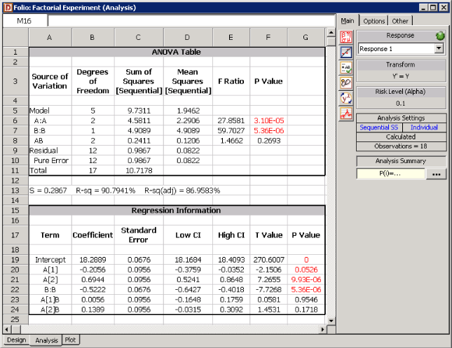
Assuming that the desired significance level is 0.1, since [math]\displaystyle{ p }[/math] value > 0.1, we fail to reject [math]\displaystyle{ {{H}_{0}}\ \ :{{(\tau \delta )}_{ij}}=0 }[/math] and conclude that the interaction between speed and fuel additive does not significantly affect the mileage of the sports utility vehicle. DOE++ displays this result in the ANOVA table, as shown in Figure FactDesingResultsSshot. In the absence of the interaction, the analysis of main effects becomes important.
The test statistic for factor [math]\displaystyle{ A }[/math] is:
- [math]\displaystyle{ \begin{align} & {{({{f}_{0}})}_{A}}= & \frac{M{{S}_{A}}}{M{{S}_{E}}} \\ & = & \frac{S{{S}_{A}}/dof(S{{S}_{A}})}{S{{S}_{E}}/dof(S{{S}_{E}})} \\ & = & \frac{4.5811/2}{0.9867/12} \\ & = & 27.86 \end{align} }[/math]
The [math]\displaystyle{ p }[/math] value corresponding to this statistic based on the [math]\displaystyle{ F }[/math] distribution with 2 degrees of freedom in the numerator and 12 degrees of freedom in the denominator is:
- [math]\displaystyle{ \begin{align} & p\text{ }value= & 1-P(F\le {{({{f}_{0}})}_{A}}) \\ & = & 1-0.99997 \\ & = & 0.00003 \end{align} }[/math]
Since [math]\displaystyle{ p }[/math] value < 0.1, [math]\displaystyle{ {{H}_{0}}\ \ :\ \ {{\tau }_{i}}=0 }[/math] is rejected and it is concluded that factor [math]\displaystyle{ A }[/math] (or speed) has a significant effect on the mileage.
The test statistic for factor [math]\displaystyle{ B }[/math] is:
- [math]\displaystyle{ \begin{align} & {{({{f}_{0}})}_{B}}= & \frac{M{{S}_{B}}}{M{{S}_{E}}} \\ & = & \frac{4.9089/1}{0.9867/12} \\ & = & 59.7 \end{align} }[/math]
The [math]\displaystyle{ p }[/math] value corresponding to this statistic based on the [math]\displaystyle{ F }[/math] distribution with 2 degrees of freedom in the numerator and 12 degrees of freedom in the denominator is:
- [math]\displaystyle{ \begin{align} & p\text{ }value= & 1-P(F\le {{({{f}_{0}})}_{B}}) \\ & = & 1-0.999995 \\ & = & 0.000005 \end{align} }[/math]
Since [math]\displaystyle{ p }[/math] value < 0.1, [math]\displaystyle{ {{H}_{0}}\ \ :\ \ {{\delta }_{j}}=0 }[/math] is rejected and it is concluded that factor [math]\displaystyle{ B }[/math] (or fuel additive type) has a significant effect on the mileage.
Therefore, it can be concluded that speed and fuel additive type affect the mileage of the vehicle significantly. The results are displayed in the ANOVA table of Figure FactDesingResultsSshot.
Calculation of Effect Coefficients
Results for the effect coefficients of the model of Eqn. (TwoFactExModelRegrVer) are displayed in the Regression Information table in Figure FactDesingResultsSshot. Calculations of the results in this table are discussed next. The effect coefficients can be calculated as follows:
- [math]\displaystyle{ \begin{align} & \hat{\beta }= & {{({{X}^{\prime }}X)}^{-1}}{{X}^{\prime }}y \\ & = & \left[ \begin{matrix} 18.2889 \\ -0.2056 \\ 0.6944 \\ -0.5222 \\ 0.0056 \\ 0.1389 \\ \end{matrix} \right] \end{align} }[/math]
- Figure 6.12: Analysis results for the experiment in Table 6.5.
Therefore, [math]\displaystyle{ \hat{\mu }=18.2889 }[/math] , [math]\displaystyle{ {{\hat{\tau }}_{1}}=-0.2056 }[/math] , [math]\displaystyle{ {{\hat{\tau }}_{2}}=0.6944 }[/math] etc. As mentioned previously, these coefficients are displayed as Intercept, A[1] and A[2] respectively depending on the name of the factor used in the experimental design. The standard error for each of these estimates is obtained using the diagonal elements of the variance-covariance matrix [math]\displaystyle{ C }[/math] .
- [math]\displaystyle{ \begin{align} & C= & {{{\hat{\sigma }}}^{2}}{{({{X}^{\prime }}X)}^{-1}} \\ & = & M{{S}_{E}}\cdot {{({{X}^{\prime }}X)}^{-1}} \\ & = & \left[ \begin{matrix} 0.0046 & 0 & 0 & 0 & 0 & 0 \\ 0 & 0.0091 & -0.0046 & 0 & 0 & 0 \\ 0 & -0.0046 & 0.0091 & 0 & 0 & 0 \\ 0 & 0 & 0 & 0.0046 & 0 & 0 \\ 0 & 0 & 0 & 0 & 0.0091 & -0.0046 \\ 0 & 0 & 0 & 0 & -0.0046 & 0.0091 \\ \end{matrix} \right] \end{align} }[/math]
For example, the standard error for [math]\displaystyle{ {{\hat{\tau }}_{1}} }[/math] is:
- [math]\displaystyle{ \begin{align} & se({{{\hat{\tau }}}_{1}})= & \sqrt{{{C}_{22}}} \\ & = & \sqrt{0.0091} \\ & = & 0.0956 \end{align} }[/math]
Then the [math]\displaystyle{ t }[/math] statistic for [math]\displaystyle{ {{\hat{\tau }}_{1}} }[/math] can be obtained as:
- [math]\displaystyle{ \begin{align} & {{t}_{0}}= & \frac{{{{\hat{\tau }}}_{1}}}{se({{{\hat{\tau }}}_{1}})} \\ & = & \frac{-0.2056}{0.0956} \\ & = & -2.1506 \end{align} }[/math]
The [math]\displaystyle{ p }[/math] value corresponding to this statistic is:
Confidence intervals on [math]\displaystyle{ {{\tau }_{1}} }[/math] can also be calculated. The 90% limits on [math]\displaystyle{ {{\tau }_{1}} }[/math] are:
- [math]\displaystyle{ \begin{align} & = & {{{\hat{\tau }}}_{1}}\pm {{t}_{\alpha /2,n-(k+1)}}\sqrt{{{C}_{22}}} \\ & = & {{\tau }_{1}}\pm {{t}_{0.05,12}}\sqrt{{{C}_{22}}} \\ & = & -0.2056\pm 0.1704 \end{align} }[/math]
Thus, the 90% limits on [math]\displaystyle{ {{\tau }_{1}} }[/math] are [math]\displaystyle{ -0.3760 }[/math] and [math]\displaystyle{ -0.0352 }[/math] respectively. Results for other coefficients are obtained in a similar manner.
Least Squares Means
The estimated mean response corresponding to the [math]\displaystyle{ i }[/math] th level of any factor is obtained using the adjusted estimated mean which is also called the least squares mean. For example, the mean response corresponding to the first level of factor [math]\displaystyle{ A }[/math] is [math]\displaystyle{ \mu +{{\tau }_{1}} }[/math] . An estimate of this is [math]\displaystyle{ \hat{\mu }+{{\hat{\tau }}_{1}} }[/math] or ( [math]\displaystyle{ 18.2889+(-0.2056)=18.0833 }[/math] ). Similarly, the estimated response at the third level of factor [math]\displaystyle{ A }[/math] is [math]\displaystyle{ \hat{\mu }+{{\hat{\tau }}_{3}} }[/math] or [math]\displaystyle{ \hat{\mu }+(-{{\hat{\tau }}_{1}}-{{\hat{\tau }}_{2}}) }[/math] or ( [math]\displaystyle{ 18.2889+(0.2056-0.6944)=17.8001 }[/math] ).
Residual Analysis
As in the case of single factor experiments, plots of residuals can also be used to check for model adequacy in factorial experiments. Box-Cox transformations are also available in DOE++ for factorial experiments.
Factorial Experiments with a Single Replicate
If a factorial experiment is run only for a single replicate then it is not possible to test hypotheses about the main effects and interactions as the error sum of squares cannot be obtained. This is because the number of observations in a single replicate equals the number of terms in the ANOVA model. Hence the model fits the data perfectly and no degrees of freedom are available to obtain the error sum of squares. For example, if the two factor experiment to study the effect of speed and fuel additive type on mileage was run only as a single replicate there would be only six response values. The model of Eqn. (TwoFactExModelRegrVer) has six terms and therefore will fit the six response values perfectly. The error sum of squares, [math]\displaystyle{ S{{S}_{E}} }[/math] , for this case will be equal to zero. In some single replicate factorial experiments it is possible to assume that the interaction effects are negligible. In this case, the interaction mean square can be used as error mean square, [math]\displaystyle{ M{{S}_{E}} }[/math] , to test hypotheses about the main effects. However, such assumptions are not applicable in all cases and should be used carefully.
Blocking
Many times a factorial experiment requires so many runs that all of them cannot be completed under homogeneous conditions. This may lead to inclusion of the effects of nuisance factors into the investigation. Nuisance factors are factors that have an effect on the response but are not of primary interest to the investigator. For example two replicates of a two-factor factorial experiment require eight runs. If four runs require the duration of one day to be completed then the total experiment will require two days to be completed. The difference in the conditions on the two days may lead to introduction of effects on the response that are not the result of the two factors being investigated. Therefore, the day is a nuisance factor for this experiment. Nuisance factors can be accounted for using blocking. In blocking, experimental runs are separated based on levels of the nuisance factor. For the case of the two-factor factorial experiment where the day is a nuisance factor, separation can be made into two groups or blocks -runs that are carried out on the first day belong to block 1, and runs that are carried out on the second day belong to block 2. Thus, within each block conditions are the same with respect to the nuisance factor. As a result, each block investigates the effects of the factors of interest, while the difference in the blocks measures the effect of the nuisance factor. For the example of the two factor factorial experiment, a possible assignment of runs to the blocks could be - one replicate of the experiment is assigned to block 1 and the second replicate is assigned to block 2 (now each block contains all possible treatment combinations). Within each block, runs are subjected to randomization (i.e. randomization is now restricted to the runs within a block). Such a design, where each block contains one complete replicate and the treatments within a block are subjected to randomization, is called randomized complete block design.
In summary, blocking should always be used to account for the effects of nuisance factors if it is not possible to hold the nuisance factor at a constant level through all of the experimental runs. Randomization should be used within each block to counter the effects of any unknown variability that may still be present.
Example 3
- Figure 6.13: Randomized complete block design for the experiment in Table 6.5 using three blocks.
Consider the experiment of Table 6.5 where the mileage of a sports utility vehicle was investigated for the effects of speed and fuel additive type. Now assume that the three replicates for this experiment were carried out on three different vehicles. To ensure that the variation from one vehicle to another does not have an effect on the analysis, each vehicle is considered as one block. (See the experiment design in Figure TwoFactBlockDesingSshot.) For the purpose of the analysis, the block is considered as a main effect except that it is assumed that interactions between the block and the other main effects do not exist. Therefore, there is one block main effect (having three levels - block 1, block 2 and block 3), two main effects (speed -having three levels; and fuel additive type - having two levels) and one interaction effect (speed-fuel additive interaction) for this experiment. Let [math]\displaystyle{ {{\zeta }_{i}} }[/math] represent the block effects. The hypothesis test on the block main effect checks if there is a significant variation from one vehicle to the other. The statements for the hypothesis test are:
- [math]\displaystyle{ \begin{align} & {{H}_{0}}: & {{\zeta }_{1}}={{\zeta }_{2}}={{\zeta }_{3}}=0\text{ (no main effect of block)} \\ & {{H}_{1}}: & {{\zeta }_{i}}\ne 0\text{ for at least one }i \end{align} }[/math]
The test statistic for this test is:
- [math]\displaystyle{ {{F}_{0}}=\frac{M{{S}_{Block}}}{M{{S}_{E}}} }[/math]
where [math]\displaystyle{ M{{S}_{Block}} }[/math] represents the mean square for the block main effect and [math]\displaystyle{ M{{S}_{E}} }[/math] is the error mean square. The hypothesis statements and test statistics to test the significance of factors [math]\displaystyle{ A }[/math] (speed), [math]\displaystyle{ B }[/math] (fuel additive) and the interaction [math]\displaystyle{ AB }[/math] (speed-fuel additive interaction) can be obtained as explained in Example 2. The ANOVA model for this example can be written as:
- [math]\displaystyle{ {{Y}_{ijk}}=\mu +{{\zeta }_{i}}+{{\tau }_{j}}+{{\delta }_{k}}+{{(\tau \delta )}_{jk}}+{{\epsilon }_{ijk}} }[/math]
where:
• [math]\displaystyle{ \mu }[/math] represents the overall mean effect
[math]\displaystyle{ {{\zeta }_{i}} }[/math] is the effect of the [math]\displaystyle{ i }[/math] th level of the block ( [math]\displaystyle{ i=1,2,3 }[/math] )
• [math]\displaystyle{ {{\tau }_{j}} }[/math] is the effect of the [math]\displaystyle{ j }[/math] th level of factor [math]\displaystyle{ A }[/math] ( [math]\displaystyle{ j=1,2,3 }[/math] )
• [math]\displaystyle{ {{\delta }_{k}} }[/math] is the effect of the [math]\displaystyle{ k }[/math] th level of factor [math]\displaystyle{ B }[/math] ( [math]\displaystyle{ k=1,2 }[/math] )
• [math]\displaystyle{ {{(\tau \delta )}_{jk}} }[/math] represents the interaction effect between [math]\displaystyle{ A }[/math] and [math]\displaystyle{ B }[/math]
• and [math]\displaystyle{ {{\epsilon }_{ijk}} }[/math] represents the random error terms (which are assumed to be normally distributed with a mean of zero and variance of [math]\displaystyle{ {{\sigma }^{2}} }[/math] )
In order to calculate the test statistics, it is convenient to express the ANOVA model of Eqn. (FactorialExpWBlock) in the form [math]\displaystyle{ y=X\beta +\epsilon }[/math] . This can be done as explained next.
Expression of the ANOVA Model as [math]\displaystyle{ y=X\beta +\epsilon }[/math]
Since the effects [math]\displaystyle{ {{\zeta }_{i}} }[/math] , [math]\displaystyle{ {{\tau }_{j}} }[/math] , [math]\displaystyle{ {{\delta }_{k}} }[/math] , and [math]\displaystyle{ {{(\tau \delta )}_{jk}} }[/math] are defined as deviations from the overall mean, the following constraints exist.
Constraints on [math]\displaystyle{ {{\zeta }_{i}} }[/math] are:
- [math]\displaystyle{ \begin{align} & \underset{i=1}{\overset{3}{\mathop \sum }}\,{{\zeta }_{i}}= & 0 \\ & \text{or }{{\zeta }_{1}}+{{\zeta }_{2}}+{{\zeta }_{3}}= & 0 \end{align} }[/math]
Therefore, only two of the [math]\displaystyle{ {{\zeta }_{i}} }[/math] effects are independent. Assuming that [math]\displaystyle{ {{\zeta }_{1}} }[/math] and [math]\displaystyle{ {{\zeta }_{2}} }[/math] are independent, [math]\displaystyle{ {{\zeta }_{3}}=-({{\zeta }_{1}}+{{\zeta }_{2}}) }[/math] . (The null hypothesis to test the significance of the blocks can be rewritten using only the independent effects as [math]\displaystyle{ {{H}_{0}}\ \ :\ \ {{\zeta }_{1}}={{\zeta }_{2}}=0 }[/math] .) In DOE++, the independent block effects, [math]\displaystyle{ {{\zeta }_{1}} }[/math] and [math]\displaystyle{ {{\zeta }_{2}} }[/math] , are displayed as Block[1] and Block[2], respectively.
Constraints on [math]\displaystyle{ {{\tau }_{j}} }[/math] are:
- [math]\displaystyle{ \begin{align} & \underset{j=1}{\overset{3}{\mathop \sum }}\,{{\tau }_{j}}= & 0 \\ & \text{or }{{\tau }_{1}}+{{\tau }_{2}}+{{\tau }_{3}}= & 0 \end{align} }[/math]
Therefore, only two of the [math]\displaystyle{ {{\tau }_{j}} }[/math] effects are independent. Assuming that [math]\displaystyle{ {{\tau }_{1}} }[/math] and [math]\displaystyle{ {{\tau }_{2}} }[/math] are independent, [math]\displaystyle{ {{\tau }_{3}}=-({{\tau }_{1}}+{{\tau }_{2}}) }[/math] . The independent effects, [math]\displaystyle{ {{\tau }_{1}} }[/math] and [math]\displaystyle{ {{\tau }_{2}} }[/math] , are displayed as A[1] and A[2], respectively.
Constraints on [math]\displaystyle{ {{\delta }_{k}} }[/math] are:
- [math]\displaystyle{ \begin{align} & \underset{k=1}{\overset{2}{\mathop \sum }}\,{{\delta }_{k}}= & 0 \\ & \text{or }{{\delta }_{1}}+{{\delta }_{2}}= & 0 \end{align} }[/math]
Therefore, only one of the [math]\displaystyle{ {{\delta }_{k}} }[/math] effects is independent. Assuming that [math]\displaystyle{ {{\delta }_{1}} }[/math] is independent, [math]\displaystyle{ {{\delta }_{2}}=-{{\delta }_{1}} }[/math] . The independent effect, [math]\displaystyle{ {{\delta }_{1}} }[/math] , is displayed as B:B.
Constraints on [math]\displaystyle{ {{(\tau \delta )}_{jk}} }[/math] are:
- [math]\displaystyle{ \begin{align} & \underset{j=1}{\overset{3}{\mathop \sum }}\,{{(\tau \delta )}_{jk}}= & 0 \\ & \text{and }\underset{k=1}{\overset{2}{\mathop \sum }}\,{{(\tau \delta )}_{jk}}= & 0 \\ & \text{or }{{(\tau \delta )}_{11}}+{{(\tau \delta )}_{21}}+{{(\tau \delta )}_{31}}= & 0 \\ & {{(\tau \delta )}_{12}}+{{(\tau \delta )}_{22}}+{{(\tau \delta )}_{32}}= & 0 \\ & \text{and }{{(\tau \delta )}_{11}}+{{(\tau \delta )}_{12}}= & 0 \\ & {{(\tau \delta )}_{21}}+{{(\tau \delta )}_{22}}= & 0 \\ & {{(\tau \delta )}_{31}}+{{(\tau \delta )}_{32}}= & 0 \end{align} }[/math]
Equations (ConstraintInteraction1) to (ConstraintInteraction) represent four constraints as only four of the five equations are independent. Therefore, only two out of the six [math]\displaystyle{ {{(\tau \delta )}_{jk}} }[/math] effects are independent. Assuming that [math]\displaystyle{ {{(\tau \delta )}_{11}} }[/math] and [math]\displaystyle{ {{(\tau \delta )}_{21}} }[/math] are independent, we can express the other four effects in terms of these effects. The independent effects, [math]\displaystyle{ {{(\tau \delta )}_{11}} }[/math] and [math]\displaystyle{ {{(\tau \delta )}_{21}} }[/math] , are displayed as A[1]B and A[2]B, respectively.
Based on the ANOVA model of Eqn. (FactorialExpWBlock) and the constraints of Eqns. (ConstraintBlock) to (ConstraintInteraction), the regression version of the ANOVA model can be obtained using indicator variables. Since the block has three levels, two indicator variables, [math]\displaystyle{ {{x}_{1}} }[/math] and [math]\displaystyle{ {{x}_{2}} }[/math] , are required, which need to be coded as shown next:
- [math]\displaystyle{ \begin{align} & \text{Block 1}: & {{x}_{1}}=1,\text{ }{{x}_{2}}=0\text{ } \\ & \text{Block 2}: & {{x}_{1}}=0,\text{ }{{x}_{2}}=1\text{ } \\ & \text{Block 3}: & {{x}_{1}}=-1,\text{ }{{x}_{2}}=-1\text{ } \end{align} }[/math]
Factor [math]\displaystyle{ A }[/math] has three levels and two indicator variables, [math]\displaystyle{ {{x}_{3}} }[/math] and [math]\displaystyle{ {{x}_{4}} }[/math] , are required:
- [math]\displaystyle{ \begin{align} & \text{Treatment Effect }{{\tau }_{1}}: & {{x}_{3}}=1,\text{ }{{x}_{4}}=0 \\ & \text{Treatment Effect }{{\tau }_{2}}: & {{x}_{3}}=0,\text{ }{{x}_{4}}=1\text{ } \\ & \text{Treatment Effect }{{\tau }_{3}}: & {{x}_{3}}=-1,\text{ }{{x}_{4}}=-1\text{ } \end{align} }[/math]
Factor [math]\displaystyle{ B }[/math] has two levels and can be represented using one indicator variable, [math]\displaystyle{ {{x}_{5}} }[/math] , as follows:
- [math]\displaystyle{ \begin{align} & \text{Treatment Effect }{{\delta }_{1}}: & {{x}_{5}}=1 \\ & \text{Treatment Effect }{{\delta }_{2}}: & {{x}_{5}}=-1 \end{align} }[/math]
The [math]\displaystyle{ AB }[/math] interaction will be represented by [math]\displaystyle{ {{x}_{3}}{{x}_{5}} }[/math] and [math]\displaystyle{ {{x}_{4}}{{x}_{5}} }[/math] . The regression version of the ANOVA model can finally be obtained as:
- [math]\displaystyle{ Y=\mu +{{\zeta }_{1}}\cdot {{x}_{1}}+{{\zeta }_{2}}\cdot {{x}_{2}}+{{\tau }_{1}}\cdot {{x}_{3}}+{{\tau }_{2}}\cdot {{x}_{4}}+{{\delta }_{1}}\cdot {{x}_{5}}+{{(\tau \delta )}_{11}}\cdot {{x}_{3}}{{x}_{5}}+{{(\tau \delta )}_{21}}\cdot {{x}_{4}}{{x}_{5}}+\epsilon }[/math]
In matrix notation this model can be expressed as:
- [math]\displaystyle{ y=X\beta +\epsilon }[/math]
or:
- [math]\displaystyle{ \left[ \begin{matrix} 17.3 \\ 18.9 \\ 17.1 \\ 18.7 \\ 19.1 \\ 18.8 \\ 17.8 \\ 18.2 \\ . \\ . \\ 18.3 \\ \end{matrix} \right]=\left[ \begin{matrix} 1 & 1 & 0 & 1 & 0 & 1 & 1 & 0 \\ 1 & 1 & 0 & 0 & 1 & 1 & 0 & 1 \\ 1 & 1 & 0 & -1 & -1 & 1 & -1 & -1 \\ 1 & 1 & 0 & 1 & 0 & -1 & -1 & 0 \\ 1 & 1 & 0 & 0 & 1 & -1 & 0 & -1 \\ 1 & 1 & 0 & -1 & -1 & -1 & 1 & 1 \\ 1 & 0 & 1 & 1 & 0 & 1 & 1 & 0 \\ 1 & 0 & 1 & 0 & 1 & 1 & 0 & 1 \\ . & . & . & . & . & . & . & . \\ . & . & . & . & . & . & . & . \\ 1 & -1 & -1 & -1 & -1 & -1 & 1 & 1 \\ \end{matrix} \right]\left[ \begin{matrix} \mu \\ {{\zeta }_{1}} \\ {{\zeta }_{2}} \\ {{\tau }_{1}} \\ {{\tau }_{2}} \\ {{\delta }_{1}} \\ {{(\tau \delta )}_{11}} \\ {{(\tau \delta )}_{21}} \\ \end{matrix} \right]+\left[ \begin{matrix} {{\epsilon }_{111}} \\ {{\epsilon }_{121}} \\ {{\epsilon }_{131}} \\ {{\epsilon }_{112}} \\ {{\epsilon }_{122}} \\ {{\epsilon }_{132}} \\ {{\epsilon }_{211}} \\ {{\epsilon }_{221}} \\ . \\ . \\ {{\epsilon }_{332}} \\ \end{matrix} \right] }[/math]
Knowing [math]\displaystyle{ y }[/math] , [math]\displaystyle{ X }[/math] and [math]\displaystyle{ \beta }[/math] , the sum of squares for the ANOVA model and the extra sum of squares for each of the factors can be calculated. These are used to calculate the mean squares that are used to obtain the test statistics.
Calculation of the Sum of Squares for the Model
The model sum of squares, [math]\displaystyle{ S{{S}_{TR}} }[/math] , for the model of Eqn. (FactorialExpWBlock) can be obtained as:
- [math]\displaystyle{ \begin{align} & S{{S}_{TR}}= & {{y}^{\prime }}[H-(\frac{1}{{{n}_{a}}\cdot {{n}_{b}}\cdot m})J]y \\ & = & {{y}^{\prime }}[H-(\frac{1}{18})J]y \\ & = & 9.9256 \end{align} }[/math]
Since seven effect terms ( [math]\displaystyle{ {{\zeta }_{1}} }[/math] , [math]\displaystyle{ {{\zeta }_{2}} }[/math] , [math]\displaystyle{ {{\tau }_{1}} }[/math] , [math]\displaystyle{ {{\tau }_{2}} }[/math] , [math]\displaystyle{ {{\delta }_{1}} }[/math] , [math]\displaystyle{ {{(\tau \delta )}_{11}} }[/math] and [math]\displaystyle{ {{(\tau \delta )}_{21}} }[/math] ) are used in the model the number of degrees of freedom associated with [math]\displaystyle{ S{{S}_{TR}} }[/math] is seven ( [math]\displaystyle{ dof(S{{S}_{TR}})=7 }[/math] ).
The total sum of squares can be calculated as:
- [math]\displaystyle{ \begin{align} & S{{S}_{T}}= & {{y}^{\prime }}[I-(\frac{1}{{{n}_{a}}\cdot {{n}_{b}}\cdot m})J]y \\ & = & {{y}^{\prime }}[H-(\frac{1}{18})J]y \\ & = & 10.7178 \end{align} }[/math]
Since there are 18 observed response values, the number of degrees of freedom associated with the total sum of squares is 17 ( [math]\displaystyle{ dof(S{{S}_{T}})=17 }[/math] ). The error sum of squares can now be obtained:
- [math]\displaystyle{ \begin{align} & S{{S}_{E}}= & S{{S}_{T}}-S{{S}_{TR}} \\ & = & 10.7178-9.9256 \\ & = & 0.7922 \end{align} }[/math]
The number of degrees of freedom associated with the error sum of squares is:
- [math]\displaystyle{ \begin{align} & dof(S{{S}_{E}})= & dof(S{{S}_{T}})-dof(S{{S}_{TR}}) \\ & = & 17-7 \\ & = & 10 \end{align} }[/math]
Since there are no true replicates of the treatments (as can be seen from the design of Figure TwoFactBlockDesingSshot where all of the treatments are seen to be run just once), all of the error sum of squares is the sum of squares due to lack of fit. The lack of fit arises because the model used is not a full model since it is assumed that there are no interactions between blocks and other effects.
Calculation of the Extra Sum of Squares for the Factors
The sequential sum of squares for the blocks can be calculated as:
- [math]\displaystyle{ \begin{align} & S{{S}_{Block}}= & S{{S}_{TR}}(\mu ,{{\zeta }_{1}},{{\zeta }_{2}})-S{{S}_{TR}}(\mu ) \\ & = & {{y}^{\prime }}[{{H}_{\mu ,{{\zeta }_{1}},{{\zeta }_{2}}}}-(\frac{1}{18})J]y-0 \end{align} }[/math]
where [math]\displaystyle{ J }[/math] is the matrix of ones, [math]\displaystyle{ {{H}_{\mu ,{{\zeta }_{1}},{{\zeta }_{2}}}} }[/math] is the hat matrix, which is calculated using [math]\displaystyle{ {{H}_{\mu ,{{\zeta }_{1}},{{\zeta }_{2}}}}={{X}_{\mu ,{{\zeta }_{1}},{{\zeta }_{2}}}}{{(X_{\mu ,{{\zeta }_{1}},{{\zeta }_{2}}}^{\prime }{{X}_{\mu ,{{\zeta }_{1}},{{\zeta }_{2}}}})}^{-1}}X_{\mu ,{{\zeta }_{1}},{{\zeta }_{2}}}^{\prime } }[/math] , and [math]\displaystyle{ {{X}_{\mu ,{{\zeta }_{1}},{{\zeta }_{2}}}} }[/math] is the matrix containing only the first three columns of the [math]\displaystyle{ X }[/math] matrix. Thus
- [math]\displaystyle{ \begin{align} & S{{S}_{Block}}= & {{y}^{\prime }}[{{H}_{\mu ,{{\zeta }_{1}},{{\zeta }_{2}}}}-(\frac{1}{18})J]y-0 \\ & = & 0.1944-0 \\ & = & 0.1944 \end{align} }[/math]
Since there are two independent block effects, and [math]\displaystyle{ {{\zeta }_{2}} }[/math] , the number of degrees of freedom associated with [math]\displaystyle{ S{{S}_{Blocks}} }[/math] is two ( [math]\displaystyle{ dof(S{{S}_{Blocks}})=2 }[/math] ).
Similarly, the sequential sum of squares for factor [math]\displaystyle{ A }[/math] can be calculated as:
- [math]\displaystyle{ \begin{align} & S{{S}_{A}}= & S{{S}_{TR}}(\mu ,{{\zeta }_{1}},{{\zeta }_{2}},{{\tau }_{1}},{{\tau }_{2}})-S{{S}_{TR}}(\mu ,{{\zeta }_{1}},{{\zeta }_{2}}) \\ & = & {{y}^{\prime }}[{{H}_{\mu ,{{\zeta }_{1}},{{\zeta }_{2}},{{\tau }_{1}},{{\tau }_{2}}}}-(\frac{1}{18})J]y-{{y}^{\prime }}[{{H}_{\mu ,{{\zeta }_{1}},{{\zeta }_{2}}}}-(\frac{1}{18})J]y \\ & = & 4.7756-0.1944 \\ & = & 4.5812 \end{align} }[/math]
Sequential sum of squares for the other effects are obtained as [math]\displaystyle{ S{{S}_{B}}=4.9089 }[/math] and [math]\displaystyle{ S{{S}_{AB}}=0.2411 }[/math] .
Calculation of the Test Statistics
Knowing the sum of squares, the test statistics for each of the factors can be calculated. For example, the test statistic for the main effect of the blocks is:
- [math]\displaystyle{ \begin{align} & {{({{f}_{0}})}_{Block}}= & \frac{M{{S}_{Block}}}{M{{S}_{E}}} \\ & = & \frac{S{{S}_{Block}}/dof(S{{S}_{Blocks}})}{S{{S}_{E}}/dof(S{{S}_{E}})} \\ & = & \frac{0.1944/2}{0.7922/10} \\ & = & 1.227 \end{align} }[/math]
The [math]\displaystyle{ p }[/math] value corresponding to this statistic based on the [math]\displaystyle{ F }[/math] distribution with 2 degrees of freedom in the numerator and 10 degrees of freedom in the denominator is:
- [math]\displaystyle{ \begin{align} & p\text{ }value= & 1-P(F\le {{({{f}_{0}})}_{Block}}) \\ & = & 1-0.6663 \\ & = & 0.3337 \end{align} }[/math]
Assuming that the desired significance level is 0.1, since [math]\displaystyle{ p }[/math] value > 0.1, we fail to reject [math]\displaystyle{ {{H}_{0}}\ \ :\ \ {{\zeta }_{i}}=0 }[/math] and conclude that there is no significant variation in the mileage from one vehicle to the other. Statistics to test the significance of other factors can be calculated in a similar manner. The complete analysis results obtained from DOE++ for this experiment are presented in Figure TwoFactBlockDesingResultsSshot.
- Figure 6.14: Analysis results for the experiment in Example 3.
Use of Regression to Calculate Sum of Squares
This section explains the reason behind the use of regression in DOE++ in all calculations related to the sum of squares. A number of textbooks present the method of direct summation to calculate the sum of squares. But this method is only applicable for balanced designs and may give incorrect results for unbalanced designs. For example, the sum of squares for factor [math]\displaystyle{ A }[/math] in a balanced factorial experiment with two factors, [math]\displaystyle{ A }[/math] and [math]\displaystyle{ B }[/math] , is given as follows:
- [math]\displaystyle{ \begin{align} & S{{S}_{A}}= & \underset{i=1}{\overset{{{n}_{a}}}{\mathop{\sum }}}\,{{n}_{b}}n{{({{{\bar{y}}}_{i..}}-{{{\bar{y}}}_{...}})}^{2}} \\ & = & \underset{i=1}{\overset{{{n}_{a}}}{\mathop{\sum }}}\,\frac{y_{i..}^{2}}{{{n}_{b}}n}-\frac{y_{...}^{2}}{{{n}_{a}}{{n}_{b}}n} \end{align} }[/math]
where [math]\displaystyle{ {{n}_{a}} }[/math] represents the levels of factor [math]\displaystyle{ A }[/math] , [math]\displaystyle{ {{n}_{b}} }[/math] represents the levels of factor [math]\displaystyle{ B }[/math] , and [math]\displaystyle{ n }[/math] represents the number of samples for each combination of [math]\displaystyle{ A }[/math] and [math]\displaystyle{ B }[/math] . The term [math]\displaystyle{ {{\bar{y}}_{i..}} }[/math] is the mean value for the [math]\displaystyle{ i }[/math] th level of factor [math]\displaystyle{ A }[/math] , [math]\displaystyle{ {{y}_{i..}} }[/math] is the sum of all observations at the [math]\displaystyle{ i }[/math] th level of factor [math]\displaystyle{ A }[/math] and [math]\displaystyle{ {{y}_{...}} }[/math] is the sum of all observations.
The analogous term to calculate [math]\displaystyle{ S{{S}_{A}} }[/math] in the case of an unbalanced design is given as:
- [math]\displaystyle{ S{{S}_{A}}=\underset{i=1}{\overset{{{n}_{a}}}{\mathop{\sum }}}\,\frac{y_{i..}^{2}}{{{n}_{i.}}}-\frac{y_{...}^{2}}{{{n}_{..}}} }[/math]
where [math]\displaystyle{ {{n}_{i.}} }[/math] is the number of observations at the [math]\displaystyle{ i }[/math] th level of factor [math]\displaystyle{ A }[/math] and [math]\displaystyle{ {{n}_{..}} }[/math] is the total number of observations. Similarly, to calculate the sum of squares for factor [math]\displaystyle{ B }[/math] and interaction [math]\displaystyle{ AB }[/math] , the formulas are given as:
- [math]\displaystyle{ \begin{align} & S{{S}_{B}}= & \underset{j=1}{\overset{{{n}_{b}}}{\mathop{\sum }}}\,\frac{y_{.j.}^{2}}{{{n}_{.j}}}-\frac{y_{...}^{2}}{{{n}_{..}}} \\ & S{{S}_{AB}}= & \underset{i=1}{\overset{{{n}_{a}}}{\mathop{\sum }}}\,\underset{j=1}{\overset{{{n}_{b}}}{\mathop{\sum }}}\,\frac{y_{ij.}^{2}}{{{n}_{ij}}}-\underset{i=1}{\overset{{{n}_{a}}}{\mathop{\sum }}}\,\frac{y_{i..}^{2}}{{{n}_{i.}}}-\underset{j=1}{\overset{{{n}_{b}}}{\mathop{\sum }}}\,\frac{y_{.j.}^{2}}{{{n}_{.j}}}+\frac{y_{...}^{2}}{{{n}_{..}}} \end{align} }[/math]
Applying these relations to the unbalanced data of Table 6.6, the sum of squares for the interaction [math]\displaystyle{ AB }[/math] is:
- [math]\displaystyle{ \begin{align} & S{{S}_{AB}}= & \underset{i=1}{\overset{{{n}_{a}}}{\mathop{\sum }}}\,\underset{j=1}{\overset{{{n}_{b}}}{\mathop{\sum }}}\,\frac{y_{ij.}^{2}}{{{n}_{ij}}}-\underset{i=1}{\overset{{{n}_{a}}}{\mathop{\sum }}}\,\frac{y_{i..}^{2}}{{{n}_{i.}}}-\underset{j=1}{\overset{{{n}_{b}}}{\mathop{\sum }}}\,\frac{y_{.j.}^{2}}{{{n}_{.j}}}+\frac{y_{...}^{2}}{{{n}_{..}}} \\ & = & \left( {{6}^{2}}+{{4}^{2}}+\frac{{{(42+6)}^{2}}}{2}+{{12}^{2}} \right)-\left( \frac{{{10}^{2}}}{2}+\frac{{{60}^{2}}}{3} \right) \\ & & -\left( \frac{{{54}^{2}}}{3}+\frac{{{16}^{2}}}{2} \right)+\frac{{{70}^{2}}}{5} \\ & = & -22 \end{align} }[/math]
which is obviously incorrect since the sum of squares cannot be negative. For a detailed discussion on this refer to [Searle].
- Table 6.6: Example of an unbalanced design.
The correct sum of squares can be calculated as shown next. The [math]\displaystyle{ y }[/math] and [math]\displaystyle{ X }[/math] matrices for the design of Table 6.6 can be written as:
- [math]\displaystyle{ y=\left[ \begin{matrix} 6 \\ 4 \\ 6 \\ 12 \\ 42 \\ \end{matrix} \right]\text{ and }X=\left[ \begin{matrix} 1 & 1 & 1 & 1 \\ 1 & 1 & -1 & -1 \\ 1 & -1 & 1 & -1 \\ 1 & -1 & -1 & 1 \\ 1 & -1 & 1 & -1 \\ \end{matrix} \right] }[/math]
Then the sum of squares for the interaction [math]\displaystyle{ AB }[/math] can be calculated as:
- [math]\displaystyle{ S{{S}_{AB}}={{y}^{\prime }}[H-(1/5)J]y-{{y}^{\prime }}[{{H}_{\tilde{\ }AB}}-(1/5)J]y }[/math]
where [math]\displaystyle{ H }[/math] is the hat matrix and [math]\displaystyle{ J }[/math] is the matrix of ones. The matrix [math]\displaystyle{ {{H}_{\tilde{\ }AB}} }[/math] can be calculated using [math]\displaystyle{ {{H}_{\tilde{\ }AB}}={{X}_{\tilde{\ }AB}}{{(X_{\tilde{\ }AB}^{\prime }{{X}_{\tilde{\ }AB}})}^{-1}}X_{\tilde{\ }AB}^{\prime } }[/math] where [math]\displaystyle{ {{X}_{\tilde{\ }AB}} }[/math] is the design matrix, [math]\displaystyle{ X }[/math] , excluding the last column that represents the interaction effect [math]\displaystyle{ AB }[/math] . Thus, the sum of squares for the interaction [math]\displaystyle{ AB }[/math] is:
- [math]\displaystyle{ \begin{align} & S{{S}_{AB}}= & {{y}^{\prime }}[H-(1/5)J]y-{{y}^{\prime }}[{{H}_{\tilde{\ }AB}}-(1/5)J]y \\ & = & 368-339.4286 \\ & = & 28.5714 \end{align} }[/math]
This is the value that is calculated by DOE++ (see Figure UnbalancedDesign1 for the experiment design and Figure UnbalancedDesign2 for the analysis).
- Figure 6.15: Unbalanced experimental design for the data in Table 6.6.
- Figure 6.16: Analysis for the unbalanced data in Table 6.6.

