Reliability Demonstration Test Design for Repairable Systems: Difference between revisions
John Leavitt (talk | contribs) |
|||
| Line 112: | Line 112: | ||
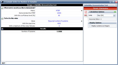
We can obtain the required number of units by using the Design of Reliability Tests (DRT) tool in the RGA software. Since this is a demonstration test then <math>\beta =1\,\!</math>, and no growth will be achieved. The results are shown next. It can be seen that in order to demonstrate a 10,000 hours MTBF with 80% confidence, 5 test units will be required. | We can obtain the required number of units by using the Design of Reliability Tests (DRT) tool in the RGA software. Since this is a demonstration test then <math>\beta =1\,\!</math>, and no growth will be achieved. The results are shown next. It can be seen that in order to demonstrate a 10,000 hours MTBF with 80% confidence, 5 test units will be required. | ||
[[Image:rga14.16.png|thumb|center| | [[Image:rga14.16.png|thumb|center|450px|Calculated number of units for the demonstration test.]] | ||
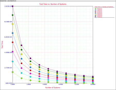
The next figure shows the different combinations of test time per unit, and the number of units in the test for different numbers of allowable failures. It helps to visually examine other possible test scenarios. | The next figure shows the different combinations of test time per unit, and the number of units in the test for different numbers of allowable failures. It helps to visually examine other possible test scenarios. | ||
[[Image:rga14.17.png|thumb|center| | [[Image:rga14.17.png|thumb|center|450px|Combinations of test time and number of units for different numbers of allowable failures.]] | ||
Revision as of 19:59, 27 November 2013
The RGA software provides a utility that allows you to design reliability demonstration tests for repairable systems. For example, you may want to design a test to demonstrate a specific cumulative MTBF for a specific operating period at a specific confidence level for a repairable system. The same applies for demonstrating an instantaneous MTBF or cumulative and instantaneous failure intensity at a given time [math]\displaystyle{ t.\,\! }[/math]
Underlying Theory
The failure process in a repairable system is considered to be a non-homogeneous Poisson process (NHPP) with power law failure intensity. The instantaneous failure intensity at time [math]\displaystyle{ t\,\! }[/math] is:
- [math]\displaystyle{ {{\lambda }_{i}}\left( t \right)=\lambda \beta {{t}^{\beta -1}}={{\lambda }_{c}}\left( t \right)\beta \,\! }[/math]
So, the cumulative failure intensity at time [math]\displaystyle{ t\,\! }[/math] is:
- [math]\displaystyle{ {{\lambda }_{c}}\left( t \right)=\lambda {{t}^{\beta -1}}=\frac{{{\lambda }_{i}}\left( t \right)}{\beta }\,\! }[/math]
The instantaneous MTTF is:
- [math]\displaystyle{ \begin{align} MTT{{F}_{i}}\left( t \right)= & \frac{1}{{{\lambda }_{i\left( t \right)}}} \\ = & \frac{1}{\lambda \beta }{{t}^{1-\beta }} \\ = & \frac{MTT{{F}_{c}}\left( t \right)}{\beta } \end{align}\,\! }[/math]
The cumulative MTBF at time [math]\displaystyle{ t\,\! }[/math] is:
- [math]\displaystyle{ MTB{{F}_{c}}\left( \beta \right)=\frac{1}{{{\lambda }_{c}}\left( t \right)}=\frac{1}{\lambda }{{t}^{1-\beta }}=MTT{{F}_{i}}\left( t \right)\beta \,\! }[/math]
The relation between the confidence level, required test time, number of systems under test and allowed total number of failures in the test is:
- [math]\displaystyle{ 1-CL=\underset{i=0}{\overset{r}{\mathop \sum }}\,\frac{{{\left( m\lambda {{T}^{\beta }} \right)}^{i}}\exp (-m\lambda {{T}^{\beta }})}{i!}\,\! }[/math]
where:
- [math]\displaystyle{ T\,\! }[/math] is the total test time for each system.
- [math]\displaystyle{ m\,\! }[/math] is the number of systems under test.
- [math]\displaystyle{ r\,\! }[/math] is the number of allowed failures in the test.
- [math]\displaystyle{ CL\,\! }[/math] is the confidence level.
Given any three of the parameters, the equation above can be solved for the fourth unknown parameter. Note that when [math]\displaystyle{ \beta =1,\,\! }[/math] the number of failures is a homogeneous Poisson process, and the time between failures is given by the exponential distribution.
Example: Solve for Time
The objective is to design a test to demonstrate that the number of failures per system in five years is less than or equal to 10. In other words, demonstrate that the cumulative MTBF for a repairable system is less than or equal to 0.5 during a five year operating period, with 80% confidence level. Assume that [math]\displaystyle{ \beta =1\,\! }[/math], the number of systems for the test is [math]\displaystyle{ m=6\,\! }[/math] and that the number of allowed failures in the test is [math]\displaystyle{ r=2.\,\! }[/math]
Solution
Since the given requirement is the number of failures, we transfer the requirement to the cumulative MTBF or cumulative failure intensity.
- [math]\displaystyle{ MTBF_c=\frac{5}{10}=0.5 year\,\! }[/math]
- then:
- [math]\displaystyle{ {{\lambda }_{c}}=\frac{1}{MTB{{F}_{c}}}=2\text{ }failures/\ \ year\,\! }[/math]
We can then solve for [math]\displaystyle{ \lambda \,\! }[/math] :
- [math]\displaystyle{ {{\lambda }_{c}}\left( t \right)=\lambda {{t}^{\beta -1}}\,\! }[/math]
For the five year period:
- [math]\displaystyle{ {{\lambda }_{c}}\left( 5 \right)=\lambda \cdot {{5}^{\beta -1}}\,\! }[/math]
Using the values of [math]\displaystyle{ \lambda \,\! }[/math] and [math]\displaystyle{ \beta \,\! }[/math], we have:
- [math]\displaystyle{ 2=\lambda \cdot {{5}^{1-1}}\,\! }[/math]
Then solving for [math]\displaystyle{ \lambda \,\! }[/math] yields:
- [math]\displaystyle{ \begin{align} \lambda =2 \end{align}\,\! }[/math]
We can then solve for the required test time, [math]\displaystyle{ T,\,\! }[/math] for each system:
- [math]\displaystyle{ 1-CL=\underset{i=0}{\overset{r}{\mathop \sum }}\,\frac{{{\left( m\lambda {{T}^{\beta }} \right)}^{i}}\exp (-m\lambda {{T}^{\beta }})}{i!}\,\! }[/math]
- or:
- [math]\displaystyle{ 1-0.8=\underset{i=0}{\overset{2}{\mathop \sum }}\,\frac{{{\left( 6\cdot 0.894\cdot {{T}^{1}} \right)}^{i}}\exp (-6\cdot 2\cdot {{T}^{1}})}{i!}\,\! }[/math]
- or:
- [math]\displaystyle{ 0.2=exp (-6\cdot 2\cdot T^1)+\,\! }[/math]
- [math]\displaystyle{ \frac{(6\cdot 2\cdot T^1)^1 exp(-6\cdot 2\cdot T^1)}{1!}\,\! }[/math]
- [math]\displaystyle{ +\frac{6\cdot 2\cdot T^1)^2 exp(-6\cdot 2\cdot T^1)}{2!}\,\! }[/math]
- [math]\displaystyle{ \frac{(6\cdot 2\cdot T^1)^1 exp(-6\cdot 2\cdot T^1)}{1!}\,\! }[/math]
- [math]\displaystyle{ 0.2=exp (-6\cdot 2\cdot T^1)+\,\! }[/math]
Solving the above equation numerically yields:
- [math]\displaystyle{ \begin{align} T=0.36 \end{align}\,\! }[/math]
In other words, for this example we have to test for 0.36 years to demonstrate that the number of failures per system in five years is less than or equal to 10.
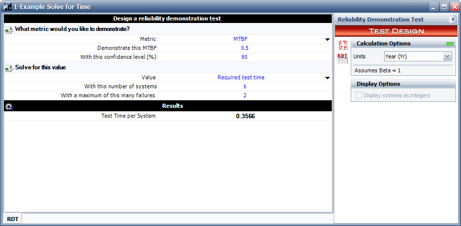
The same result can be obtained in the RGA software, by using the Design of Reliability Tests (DRT) tool. The next figure shows the calculated required test time per system of 0.3566 on the results of the example.

Example: Solve for Number of Samples
At the end of a reliability growth testing program, a manufacturer wants to demonstrate that a new product has achieved an MTBF of 10,000 hours with 80% confidence. The available time for the demonstration test is 4,000 hours for each test unit. Assuming zero failures are allowed, what is the required number of units to be tested in order to demonstrate the desired MTBF?
Solution
We can obtain the required number of units by using the Design of Reliability Tests (DRT) tool in the RGA software. Since this is a demonstration test then [math]\displaystyle{ \beta =1\,\! }[/math], and no growth will be achieved. The results are shown next. It can be seen that in order to demonstrate a 10,000 hours MTBF with 80% confidence, 5 test units will be required.
The next figure shows the different combinations of test time per unit, and the number of units in the test for different numbers of allowable failures. It helps to visually examine other possible test scenarios.


