Highly Fractional Factorial Designs

This chapter discusses factorial designs that are commonly used in designed experiments, but are not necessarily limited to two level factors. These designs are the Plackett-Burman designs and Taguchi's orthogonal arrays.

Plackett-Burman Designs

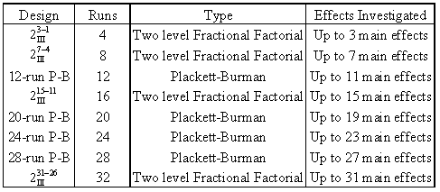
It was mentioned in Two Level Factorial Experiments that resolution III designs can be used as highly fractional designs to investigate [math]\displaystyle{ k\,\! }[/math] main effects using [math]\displaystyle{ k+1\,\! }[/math] runs (provided that three factor and higher order interaction effects are not important to the experimenter). A limitation with these designs is that all runs in these designs have to be a power of 2. The valid runs for these designs are 4, 8, 16, 32, etc. Therefore, the next design after the 2 [math]\displaystyle{ _{\text{III}}^{3-1}\,\! }[/math] design with 4 runs is the 2 [math]\displaystyle{ _{\text{III}}^{7-4}\,\! }[/math] design with 8 runs, and the design after this is the 2 [math]\displaystyle{ _{\text{III}}^{15-11}\,\! }[/math] design with 32 runs and so on, as shown in the next table.

Highly fractional designs to investigate main effects.

Plackett-Burman designs solve this problem. These designs were proposed by R. L. Plackett and J.P. Burman (1946). They allow the estimation of [math]\displaystyle{ k\,\! }[/math] main effects using [math]\displaystyle{ k+1\,\! }[/math] runs. In these designs, runs are a multiple of 4 (i.e., 4, 8, 12, 16, 20 and so on). When the runs are a power of 2, the designs correspond to the resolution III two factor fractional factorial designs. Although Plackett-Burman designs are all two level orthogonal designs, the alias structure for these designs is complicated when runs are not a power of 2.

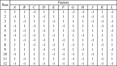
As an example, consider the 12-run Plackett-Burman design shown in the figure below.

12-run Plackett-Burman design.

If 11 main effects are to be estimated using this design, then each of these main effects is partially aliased with all other two factor interactions not containing that main effect. For example, the main effect [math]\displaystyle{ A\,\! }[/math] is partially aliased with all two factor interactions except [math]\displaystyle{ AB\,\! }[/math], [math]\displaystyle{ AC\,\! }[/math], [math]\displaystyle{ AD\,\! }[/math], [math]\displaystyle{ AE\,\! }[/math], [math]\displaystyle{ AF\,\! }[/math], [math]\displaystyle{ AG\,\! }[/math], [math]\displaystyle{ AH\,\! }[/math], [math]\displaystyle{ AJ\,\! }[/math], [math]\displaystyle{ AK\,\! }[/math] and [math]\displaystyle{ AL\,\! }[/math]. There are 45 such two factor interactions that are aliased with [math]\displaystyle{ A\,\! }[/math].

[math]\displaystyle{ \begin{align} & A= & A-\frac{1}{3}BC-\frac{1}{3}BD+\frac{1}{3}CD-\frac{1}{3}BE-\frac{1}{3}CE+\frac{1}{3}DE+... \\ & & ...+\frac{1}{3}EL-\frac{1}{3}FL-\frac{1}{3}GL+\frac{1}{3}HL+\frac{1}{3}JL-\frac{1}{3}KL \end{align}\,\! }[/math]

Due to the complex aliasing, Plackett-Burman designs involving a large number of factors should be used with care. Some of the Plackett-Burman designs available in DOE++ are included in Appendix C.

Taguchi's Orthogonal Arrays

Taguchi's orthogonal arrays are highly fractional orthogonal designs proposed by Dr. Genichi Taguchi, a Japanese industrialist. These designs can be used to estimate main effects using only a few experimental runs. These designs are not only applicable to two level factorial experiments; they can also investigate main effects when factors have more than two levels. Designs are also available to investigate main effects for certain mixed level experiments where the factors included do not have the same number of levels. As in the case of Placket-Burman designs, these designs require the experimenter to assume that interaction effects are unimportant and can be ignored. A few of Taguchi's orthogonal arrays available in DOE++ are included in Appendix D.

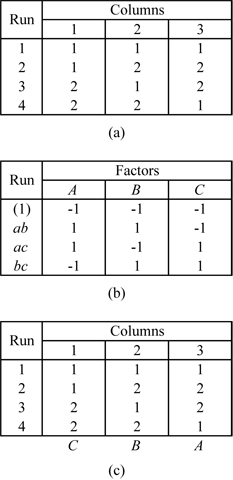
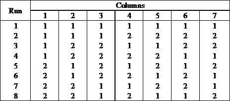
Some of Taguchi's arrays, with runs that are a power of 2, are similar to the corresponding 2 [math]\displaystyle{ _{\text{III}}^{k-f}\,\! }[/math] designs. For example, consider the L4 array shown in figure (a) below. The L4 array is denoted as L4(2^3) in DOE++. L4 means the array requires 4 runs. 2^3 indicates that the design estimates up to three main effects at 2 levels each. The L4 array can be used to estimate three main effects using four runs provided that the two factor and three factor interactions can be ignored. Figure (b) below shows the 2 [math]\displaystyle{ _{\text{III}}^{3-1}\,\! }[/math] design (defining relation [math]\displaystyle{ I=-ABC\,\! }[/math] ) which also requires four runs and can be used to estimate up to three main effects, assuming that all two factor and three factor interactions are unimportant. A comparison between the two designs shows that the columns in the two designs are the same except for the arrangement of the columns. In figure (c) below, columns of the L4 array are marked with the name of the effect from the corresponding column of the 2 [math]\displaystyle{ _{\text{III}}^{3-1}\,\! }[/math] design.

Taguchi's L4 orthogonal array - Figure (a) shows the design, (b) shows the [math]\displaystyle{ 2_{III}^{3-1} \,\! }[/math] design with the defining relation [math]\displaystyle{ I=-ABC \,\! }[/math] and (c) marks the columns of the L4 array with the corresponding columns of the design in (b).

Similarly, consider the L8(2^7) array shown in figure (a) below. This design can be used to estimate up to seven main effects using eight runs. This array is again similar to the 2 [math]\displaystyle{ _{\text{III}}^{7-4}\,\! }[/math] design shown in figure (b) below, except that the aliasing between the columns of the two designs differs in sign for some of the columns (see figure (c)).

Taguchi's L8 orthogonal array - Figure (a) shows the design, (b) shows the [math]\displaystyle{ 2_{III}^{7-4} \,\! }[/math] design with the defining relation [math]\displaystyle{ I=ABD=ACE=BCF=ABCG \,\! }[/math] and (c) marks the columns of the L8 array with the corresponding columns of the design in (b).

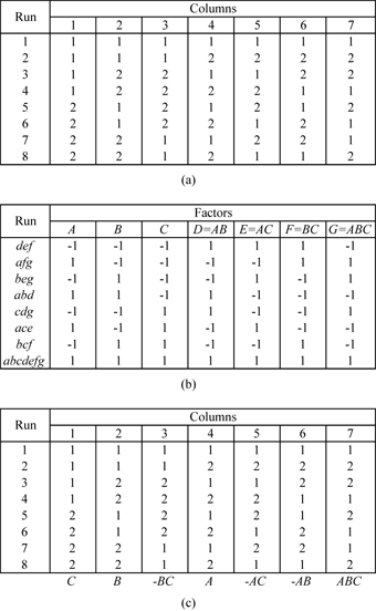
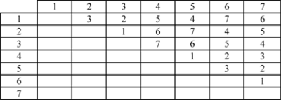
The L8 array can also be used as a full factorial three factor experiment design in the same way as a [math]\displaystyle{ 2^{3}\,\! }[/math] design. However, the orthogonal arrays should be used carefully in such cases, taking into consideration the alias relationships between the columns of the array. For the L8 array, figure (c) above shows that the third column of the array is the product of the first two columns. If the L8 array is used as a two level full factorial design in the place of a 2 [math]\displaystyle{ ^{3}\,\! }[/math] design, and if the main effects are assigned to the first three columns, the main effect assigned to the third column will be aliased with the two factor interaction of the first two main effects. The proper assignment of the main effects to the columns of the L8 array requires the experimenter to assign the three main effects to the first, second and fourth columns. These columns are sometimes referred to as the preferred columns for the L8 array. To know the preferred columns for any of the orthogonal arrays, the alias relationships between the array columns must be known. The alias relations between the main effects and two factor interactions of the columns for the L8 array are shown in the next table.

Alias relations for the L8 array.

The cell value in any ([math]\displaystyle{ i,j\,\! }[/math]) cell of the table gives the column number of the two factor interaction for the [math]\displaystyle{ i\,\! }[/math]th row and [math]\displaystyle{ j\,\! }[/math]th column. For example, to know which column is confounded with the interaction of the first and second columns, look at the value in the ( [math]\displaystyle{ 1,2\,\! }[/math] ) cell. The value of 3 indicates that the third column is the same as the product of the first and second columns. The alias relations for some of Taguchi's orthogonal arrays are available in Appendix E.

Example

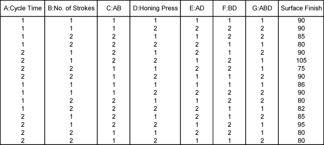
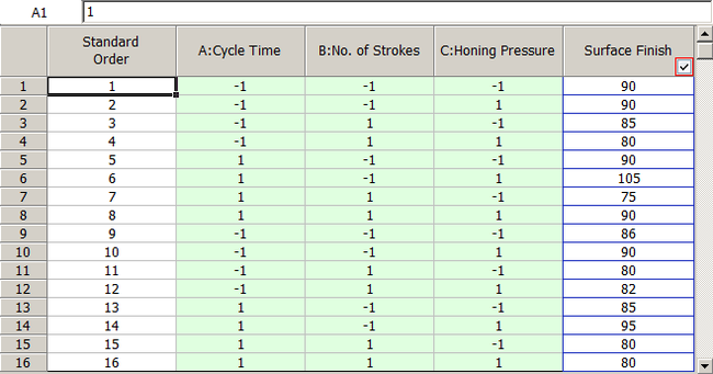
Recall the experiment to investigate factors affecting the surface finish of automobile brake drums discussed in Two Level Factorial Experiments. The three factors investigated in the experiment were honing pressure (factor A), number of strokes (factor B) and cycle time (factor C). Assume that you used Taguchi's L8 orthogonal array to investigate the three factors instead of the [math]\displaystyle{ {2}^{3}\,\! }[/math] design that was used in Two Level Factorial Experiments. Based on the discussion in the previous section, the preferred columns for the L8 array are the first, second and fourth columns. Therefore, the three factors should be assigned to these columns. The three factors are assigned to these columns based on the figure (c) above, so that you can easily compare results obtained from the L8 array to the ones included in Two Level Factorial Experiments. Based on this assignment, the L8 array for the two replicates, along with the respective response values, should be as shown in the third table. Note that to run the experiment using the L8 array, you would use only the first, the second and the fourth column to set the three factors.

Using Taguchi's L8 array to investigate factors affecting the surface finish of automobile brake drums.

The experiment design for this example can be set using the properties shown in the figure below.

Design properties for the experiment in the example.

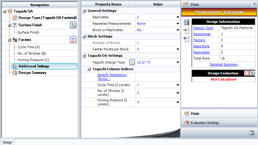
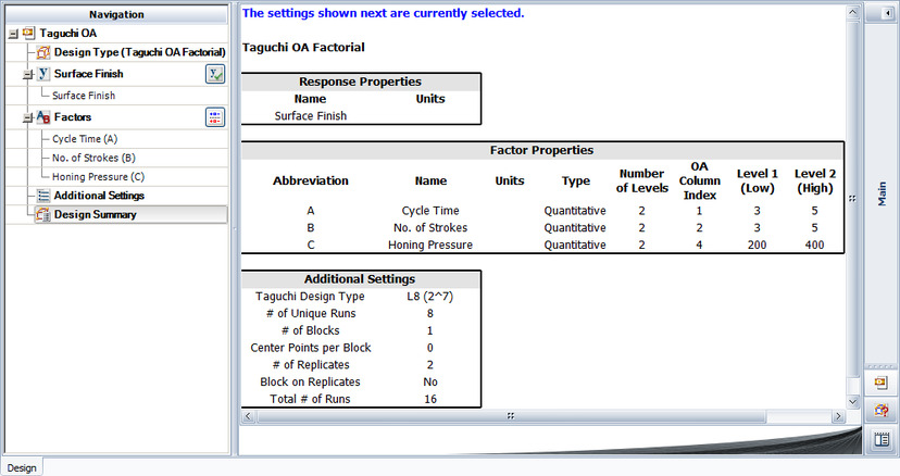
Note that for this design, the factor properties are set up as shown in the design summary.

Factor properties for the experiment in the example.

The resulting design along with the response values is shown in the figure below.

Experiment design for the example.

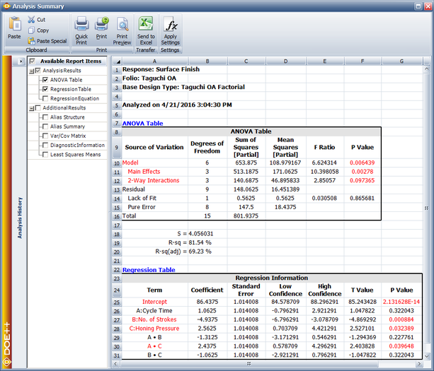
And the results from DOE++ for the design are shown in the next figure.

Results for the experiment in the example.

The results identify honing pressure, number of strokes, and the interaction between honing pressure and cycle time to be significant effects. This is identical to the conclusion obtained from the [math]\displaystyle{ {2}^{3}\,\! }[/math] design used in Two Level Factorial Experiments.

Preferred Columns in Taguchi OA

One of the difficulties of using Taguchi OA is to assign factors to the appropriate columns of the array. For example, take a simple Taguchi OA L8(2^7), which can be used for experiments with up to 7 factors. If you have only 3 factors, which 3 columns in this array should be used? DOE++ provides a simple utility to help users utilize Taguchi OA more effectively by assigning factors to the appropriate columns. Let’s use Taguchi OA L8(2^7) as an example. The design table for this array is:

This is a fractional factorial design for 7 factors. For any fractional factorial design, the first thing we need to do is check its alias structure. In general, the alias structures for Taguchi OAs are very complicated. People usually use the following table to represent the alias relations between each factor. For the above orthogonal array, the alias table is:

1	2	3	4	5	6	7
2x3	1x3	1x2	1x5	1x4	1x7	1x6
4x5	4x6	4x7	2x6	2x7	2x4	2x5
6x7	5x7	5x6	3x7	3x6	3x5	3x4

In the above table, an Arabic number is used to represent a factor. For instance, “1” represents the factor assigned to the 1st column in the array. “2x3” represents the interaction effect of the two factors assigned to column 2 and 3. Each column in the above alias table lists all the 2-way interaction effects that are aliased with the main effect of the factor assigned to this column. For example, for the 1st column, the main effect of the factor assigned to it is aliased with interaction effects of 2x3, 4x5 and 6x7. If an experiment has only 3 factors and these 3 factors A, B and C are assigned to the first 3 columns of the above L8(2^7) array, then the design table will be:

Run	A (Column 1)	B (Column 2)	C (Column 3)
1	1	1	1
2	1	1	1
3	1	2	2
4	1	2	2
5	2	1	2
6	2	1	2
7	2	2	1
8	2	2	1

The alias structure for the above table is:

[I] = I – ABC

[A] = A – BC

[B] = B – AC

[C] = C – AB

This is a resolution 3 design. All the main effects are aliased with 2-way interactions. There are many ways to choose 3 columns from the 7 columns of L8(2^7). If the 3 factors are assigned to column 1, 2, and 4, then the design table is:

Run	A (Column 1)	B (Column 2)	C (Column 4)
1	1	1	1
2	1	1	1
3	1	2	2
4	1	2	2
5	2	1	2
6	2	1	2
7	2	2	1
8	2	2	1

For experiments using the above design table, all the effects will be alias free. Therefore, this design is much better than the previous one which used column 1, 2, and 3 of L8(2^7). Although both designs have the same number of runs, more information can be obtained from this design since it is alias free.

Clearly, it is very important to assign factors to the right columns when applying Taguchi OA. DOE++ can help users automatically choose the right columns when the number of factors is less than the number of columns in a Taguchi OA. The selection is based on the specified model terms by users. Let’s use an example to explain this.

Example: Design an experiment with 3 qualitative factors. Factors A and B have 2 levels; factor C has 4 levels. The experimenters are interested in all the main effects and the interaction effect AC.

Based on this requirement, Taguchi OA L16(2^6*4^3) can be used since it can handle both 2 level and 4 level factors. It has 9 columns. The first 6 columns are used for 2 level factors and the last 3 columns are used for 4 level factors. We need assign factor A and B to two of the first 6 columns, and assign factor C to one of the last 3 columns.

In DOE++, we can choose L16(2^6*4^3) in the following window.

Click Taguchi Preferred Columns to specify the interaction terms of interest by the experimenters.

Based on the specified interaction effects, DOE++ will assign each factor to the appropriate column. In this case, they are column 1, 3, and 7 as shown below.

However, for a given Taguchi OA, it may not be possible to estimate all the specified interaction terms. If not all the requirements can be satisfied, DOE++ will assign factors to columns that result in the least number of aliased effects. In this case, users should either use another Taguchi OA or other design types. The following example is one of these cases.

Example: Design an experiment for a test with 4 qualitative factors. Factors A and B have 2 levels; C and D have 4 levels. We are interested in all the main effects and the interaction effects AC and BD.

Assume again we want to use Taguchi OA L16(2^6*4^3). Click Taguchi Preferred Columns in the following screen.

Specify the interaction effects that you want to estimate in the experiment.

When click on OK, you will get a warning message saying that it is impossible to clearly estimate all the main effects and the specified interaction effect AC and BD.

This can be explained by checking the alias table of a L16(2^6*4^3) design as given below.

1	2	3	4	5	6	7	8	9
2x7	1x7	1x9	1x5	1x4	1x8	1x2	1x6	1x3
3x9	3x6	2x6	2x8	2x9	2x3	1x8	1x7	1x7
4x5	4x8	4x7	3x7	3x8	4x9	1x9	1x9	1x8
6x8	5x9	5x8	6x9	6x7	5x7	2x8	2x4	2x5
7x8	7x8	7x8	7x8	7x8	7x8	2x9	2x7	2x7
7x9	7x9	7x9	7x9	7x9	7x9	3x8	2x9	2x8
8x9	8x9	8x9	8x9	8x9	8x9	3x9	3x5	3x7
						4x8	3x7	3x8
						4x9	3x9	4x6
						5x6	4x7	4x7
						5x8	4x9	4x8
						5x9	5x7	5x7
						6x8	5x9	5x8
						6x9	6x7	6x7
						8x9	6x9	6x8
							7x9	7x8

From this table, we can see that it is impossible to clearly estimate both AC and BD. Factors C and D can only be assigned to the last three columns since they are 4 level factors. Assume we assign factor C to column 7 and factor D to column 8. Factor B (2 level) will be in one of the columns from 1 to 6. Therefore, effect BD will be one of the effects highlighted in the table, where the first term of the interaction is between 1 and 6 and the last term is 8 (i.e., factor D).

The above alias table shows factor C is aliased with one of those highlighted effects. Thus, no matter which of the first six columns is assigned to factor B, the main effect C will be aliased with interaction effect BD. This is also true if C is assigned to column 8 or 9. Therefore, if L16(2^6*4^3) is used, there is no way to clearly estimate all the main effects and the interaction effects AC and BD. Another Taguchi OA or other design types such as a general level full factorial design should be used. A more efficient way probably is to create an optimal custom design that can clearly estimate all the specified terms. For more detail, please refer to the chapter on Optimal Custom Designs.