General Full Factorial Designs: Difference between revisions
Chris Kahn (talk | contribs) No edit summary |
Chris Kahn (talk | contribs) No edit summary |
||
| Line 631: | Line 631: | ||
===Residual Analysis=== | ===Residual Analysis=== | ||
As in the case of single factor experiments, plots of residuals can also be used to check for model adequacy in factorial experiments. Box-Cox transformations are also available in DOE++ for factorial experiments. | As in the case of single factor experiments, plots of residuals can also be used to check for model adequacy in factorial experiments. Box-Cox transformations are also available in DOE++ for factorial experiments. | ||
Revision as of 19:20, 30 January 2013
Experiments with two or more factors are encountered frequently. The best way to carry out such experiments is by using factorial experiments. Factorial experiments are experiments in which all combinations of factors are investigated in each replicate of the experiment. Factorial experiments are the only means to completely and systematically study interactions between factors in addition to identifying significant factors. One-factor-at-a-time experiments (where each factor is investigated separately by keeping all the remaining factors constant) do not reveal the interaction effects between the factors. Further, in one-factor-at-a-time experiments full randomization is not possible.
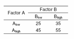
To illustrate factorial experiments consider an experiment where the response is investigated for two factors, [math]\displaystyle{ A\,\! }[/math] and [math]\displaystyle{ B\,\! }[/math]. Assume that the response is studied at two levels of factor [math]\displaystyle{ A\,\! }[/math] with [math]\displaystyle{ {{A}_{\text{low}}}\,\! }[/math] representing the lower level of [math]\displaystyle{ A\,\! }[/math] and [math]\displaystyle{ {{A}_{\text{high}}}\,\! }[/math] representing the higher level of [math]\displaystyle{ A\,\! }[/math]. Similarly, let [math]\displaystyle{ {{B}_{\text{low}}}\,\! }[/math] and [math]\displaystyle{ {{B}_{\text{high}}}\,\! }[/math] represent the two levels of factor [math]\displaystyle{ B\,\! }[/math] that are being investigated in this experiment. Since there are two factors with two levels, a total of [math]\displaystyle{ 2\times 2=4\,\! }[/math] combinations exist ([math]\displaystyle{ {{A}_{\text{low}}}\,\! }[/math] - [math]\displaystyle{ {{B}_{\text{low}}}\,\! }[/math], - [math]\displaystyle{ {{B}_{\text{high}}}\,\! }[/math], [math]\displaystyle{ {{A}_{\text{high}}}\,\! }[/math] - [math]\displaystyle{ {{B}_{\text{low}}}\,\! }[/math], - [math]\displaystyle{ {{B}_{\text{high}}}\,\! }[/math]). Thus, four runs are required for each replicate if a factorial experiment is to be carried out in this case. Assume that the response values for each of these four possible combinations are obtained as shown in the third table.
Investigating Factor Effects
The effect of factor [math]\displaystyle{ A\,\! }[/math] on the response can be obtained by taking the difference between the average response when [math]\displaystyle{ A\,\! }[/math] is high and the average response when [math]\displaystyle{ A\,\! }[/math] is low. The change in the response due to a change in the level of a factor is called the main effect of the factor. The main effect of [math]\displaystyle{ A\,\! }[/math] as per the response values in the third table is:
- [math]\displaystyle{ \begin{align} A= & Average\text{ }response\text{ }at\text{ }{{A}_{\text{high}}}-Average\text{ }response\text{ }at\text{ }{{A}_{\text{low}}} \\ = & \frac{45+55}{2}-\frac{25+35}{2} \\ = & 50-30 \\ = & 20 \end{align}\,\! }[/math]
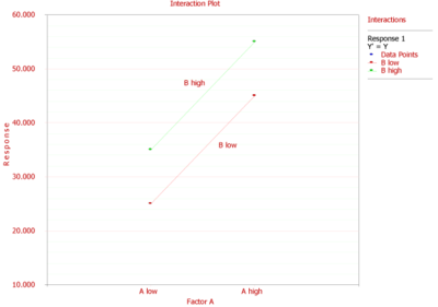
Therefore, when [math]\displaystyle{ A\,\! }[/math] is changed from the lower level to the higher level, the response increases by 20 units. A plot of the response for the two levels of [math]\displaystyle{ A\,\! }[/math] at different levels of [math]\displaystyle{ B\,\! }[/math] is shown in the figure above. The plot shows that change in the level of [math]\displaystyle{ A\,\! }[/math] leads to an increase in the response by 20 units regardless of the level of [math]\displaystyle{ B\,\! }[/math]. Therefore, no interaction exists in this case as indicated by the parallel lines on the plot. The main effect of [math]\displaystyle{ B\,\! }[/math] can be obtained as:
- [math]\displaystyle{ \begin{align} B= & Average\text{ }response\text{ }at\text{ }{{B}_{\text{high}}}-Average\text{ }response\text{ }at\text{ }{{B}_{\text{low}}} \\ = & \frac{35+55}{2}-\frac{25+45}{2} \\ = & 45-35 \\ = & 10 \end{align}\,\! }[/math]
Investigating Interactions
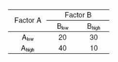
Now assume that the response values for each of the four treatment combinations were obtained as shown in the fourth table. The main effect of [math]\displaystyle{ A\,\! }[/math] in this case is:
- [math]\displaystyle{ \begin{align} A= & Average\text{ }response\text{ }at\text{ }{{A}_{\text{high}}}-Average\text{ }response\text{ }at\text{ }{{A}_{\text{low}}} \\ = & \frac{40+10}{2}-\frac{20+30}{2} \\ = & 0 \end{align}\,\! }[/math]
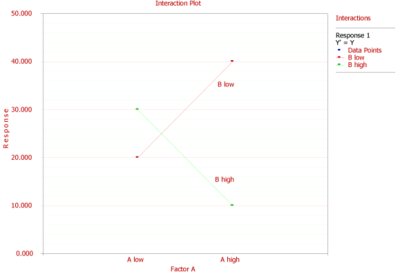
It appears that [math]\displaystyle{ A\,\! }[/math] does not have an effect on the response. However, a plot of the response of [math]\displaystyle{ A\,\! }[/math] at different levels of [math]\displaystyle{ B\,\! }[/math] shows that the response does change with the levels of [math]\displaystyle{ A\,\! }[/math] but the effect of [math]\displaystyle{ A\,\! }[/math] on the response is dependent on the level of [math]\displaystyle{ B\,\! }[/math] (see the figure below). Therefore, an interaction between [math]\displaystyle{ A\,\! }[/math] and [math]\displaystyle{ B\,\! }[/math] exists in this case (as indicated by the non-parallel lines of the figure). The interaction effect between [math]\displaystyle{ A\,\! }[/math] and [math]\displaystyle{ B\,\! }[/math] can be calculated as follows:
- [math]\displaystyle{ \begin{align} AB= & Average\text{ }response\text{ }at\text{ }{{A}_{\text{high}}}\text{-}{{B}_{\text{high}}}\text{ }and\text{ }{{A}_{\text{low}}}\text{-}{{B}_{\text{low}}}- \\ & Average\text{ }response\text{ }at\text{ }{{A}_{\text{low}}}\text{-}{{B}_{\text{high}}}\text{ }and\text{ }{{A}_{\text{high}}}\text{-}{{B}_{\text{low}}} \\ = & \frac{10+20}{2}-\frac{40+30}{2} \\ = & -20 \end{align}\,\! }[/math]
Note that in this case, if a one-factor-at-a-time experiment were used to investigate the effect of factor [math]\displaystyle{ A\,\! }[/math] on the response, it would lead to incorrect conclusions. For example, if the response at factor [math]\displaystyle{ A\,\! }[/math] was studied by holding [math]\displaystyle{ B\,\! }[/math] constant at its lower level, then the main effect of [math]\displaystyle{ A\,\! }[/math] would be obtained as [math]\displaystyle{ 40-20=20\,\! }[/math], indicating that the response increases by 20 units when the level of [math]\displaystyle{ A\,\! }[/math] is changed from low to high. On the other hand, if the response at factor [math]\displaystyle{ A\,\! }[/math] was studied by holding [math]\displaystyle{ B\,\! }[/math] constant at its higher level than the main effect of [math]\displaystyle{ A\,\! }[/math] would be obtained as [math]\displaystyle{ 10-30=-20\,\! }[/math], indicating that the response decreases by 20 units when the level of [math]\displaystyle{ A\,\! }[/math] is changed from low to high.
Analysis of General Factorial Experiments
In DOE++, factorial experiments are referred to as factorial designs. The experiments explained in this section are referred to as general factorial designs. This is done to distinguish these experiments from the other factorial designs supported by DOE++ (see the figure below).
The other designs (such as the two level full factorial designs that are explained in Two Level Factorial Experiments) are special cases of these experiments in which factors are limited to a specified number of levels. The ANOVA model for the analysis of factorial experiments is formulated as shown next. Assume a factorial experiment in which the effect of two factors, [math]\displaystyle{ A\,\! }[/math] and [math]\displaystyle{ B\,\! }[/math], on the response is being investigated. Let there be [math]\displaystyle{ {{n}_{a}}\,\! }[/math] levels of factor [math]\displaystyle{ A\,\! }[/math] and [math]\displaystyle{ {{n}_{b}}\,\! }[/math] levels of factor [math]\displaystyle{ B\,\! }[/math]. The ANOVA model for this experiment can be stated as:
- [math]\displaystyle{ {{Y}_{ijk}}=\mu +{{\tau }_{i}}+{{\delta }_{j}}+{{(\tau \delta )}_{ij}}+{{\epsilon }_{ijk}}\,\! }[/math]
where:
- [math]\displaystyle{ \mu \,\! }[/math] represents the overall mean effect
- [math]\displaystyle{ {{\tau }_{i}}\,\! }[/math] is the effect of the [math]\displaystyle{ i\,\! }[/math]th level of factor [math]\displaystyle{ A\,\! }[/math] ([math]\displaystyle{ i=1,2,...,{{n}_{a}}\,\! }[/math])
- [math]\displaystyle{ {{\delta }_{j}}\,\! }[/math] is the effect of the [math]\displaystyle{ j\,\! }[/math]th level of factor [math]\displaystyle{ B\,\! }[/math] ([math]\displaystyle{ j=1,2,...,{{n}_{b}}\,\! }[/math])
- [math]\displaystyle{ {{(\tau \delta )}_{ij}}\,\! }[/math] represents the interaction effect between [math]\displaystyle{ A\,\! }[/math] and [math]\displaystyle{ B\,\! }[/math]
- [math]\displaystyle{ {{\epsilon }_{ijk}}\,\! }[/math] represents the random error terms (which are assumed to be normally distributed with a mean of zero and variance of [math]\displaystyle{ {{\sigma }^{2}}\,\! }[/math])
- and the subscript [math]\displaystyle{ k\,\! }[/math] denotes the [math]\displaystyle{ m\,\! }[/math] replicates ([math]\displaystyle{ k=1,2,...,m\,\! }[/math])
Since the effects [math]\displaystyle{ {{\tau }_{i}}\,\! }[/math], [math]\displaystyle{ {{\delta }_{j}}\,\! }[/math] and [math]\displaystyle{ {{(\tau \delta )}_{ij}}\,\! }[/math] represent deviations from the overall mean, the following constraints exist:
- [math]\displaystyle{ \underset{i=1}{\overset{{{n}_{a}}}{\mathop \sum }}\,{{\tau }_{i}}=0\,\! }[/math]
- [math]\displaystyle{ \underset{j=1}{\overset{{{n}_{b}}}{\mathop \sum }}\,{{\delta }_{j}}=0\,\! }[/math]
- [math]\displaystyle{ \underset{i=1}{\overset{{{n}_{a}}}{\mathop \sum }}\,{{(\tau \delta )}_{ij}}=0\,\! }[/math]
- [math]\displaystyle{ \underset{j=1}{\overset{{{n}_{b}}}{\mathop \sum }}\,{{(\tau \delta )}_{ij}}=0\,\! }[/math]
Hypothesis Tests in General Factorial Experiments
These tests are used to check whether each of the factors investigated in the experiment is significant or not. For the previous example, with two factors, [math]\displaystyle{ A\,\! }[/math] and [math]\displaystyle{ B\,\! }[/math], and their interaction, [math]\displaystyle{ AB\,\! }[/math], the statements for the hypothesis tests can be formulated as follows:
- [math]\displaystyle{ \begin{align} & \begin{matrix} 1. & {} \\ \end{matrix}{{H}_{0}}:{{\tau }_{1}}={{\tau }_{2}}=...={{\tau }_{{{n}_{a}}}}=0\text{ (Main effect of }A\text{ is absent)} \\ & \begin{matrix} {} & {} \\ \end{matrix}{{H}_{1}}:{{\tau }_{i}}\ne 0\text{ for at least one }i \\ & \begin{matrix} 2. & {} \\ \end{matrix}{{H}_{0}}:{{\delta }_{1}}={{\delta }_{2}}=...={{\delta }_{{{n}_{b}}}}=0\text{ (Main effect of }B\text{ is absent)} \\ & \begin{matrix} {} & {} \\ \end{matrix}{{H}_{1}}:{{\delta }_{j}}\ne 0\text{ for at least one }j \\ & \begin{matrix} 3. & {} \\ \end{matrix}{{H}_{0}}:{{(\tau \delta )}_{11}}={{(\tau \delta )}_{12}}=...={{(\tau \delta )}_{{{n}_{a}}{{n}_{b}}}}=0\text{ (Interaction }AB\text{ is absent)} \\ & \begin{matrix} {} & {} \\ \end{matrix}{{H}_{1}}:{{(\tau \delta )}_{ij}}\ne 0\text{ for at least one }ij \end{align}\,\! }[/math]
The test statistics for the three tests are as follows:
- 1)[math]\displaystyle{ {(F_{0})}_{A} = \frac{MS_{A}}{MS_{E}}\,\! }[/math]
- where [math]\displaystyle{ MS_{A}\,\! }[/math] is the mean square due to factor [math]\displaystyle{ {A}\,\! }[/math] and [math]\displaystyle{ {MS_E}\,\! }[/math] is the error mean square.
- 1)[math]\displaystyle{ {(F_{0})}_{A} = \frac{MS_{A}}{MS_{E}}\,\! }[/math]
- 2)[math]\displaystyle{ {(F_{0})_{B}} = \frac{MS_B}{MS_E}\,\! }[/math]
- where [math]\displaystyle{ MS_{B}\,\! }[/math] is the mean square due to factor [math]\displaystyle{ B\,\! }[/math] and [math]\displaystyle{ MS_{E}\,\! }[/math] is the error mean square.
- 2)[math]\displaystyle{ {(F_{0})_{B}} = \frac{MS_B}{MS_E}\,\! }[/math]
- 3)[math]\displaystyle{ {(F_{0})_{AB}} = \frac{MS_{AB}}{MS_{E}}\,\! }[/math]
- where [math]\displaystyle{ MS_{AB}\,\! }[/math] is the mean square due to interaction [math]\displaystyle{ AB\,\! }[/math] and [math]\displaystyle{ MS_{E}\,\! }[/math] is the error mean square.
- 3)[math]\displaystyle{ {(F_{0})_{AB}} = \frac{MS_{AB}}{MS_{E}}\,\! }[/math]
The tests are identical to the partial [math]\displaystyle{ F\,\! }[/math] test explained in Multiple Linear Regression Analysis. The sum of squares for these tests (to obtain the mean squares) are calculated by splitting the model sum of squares into the extra sum of squares due to each factor. The extra sum of squares calculated for each of the factors may either be partial or sequential. For the present example, if the extra sum of squares used is sequential, then the model sum of squares can be written as:
- [math]\displaystyle{ S{{S}_{TR}}=S{{S}_{A}}+S{{S}_{B}}+S{{S}_{AB}}\,\! }[/math]
where [math]\displaystyle{ S{{S}_{TR}}\,\! }[/math] represents the model sum of squares, [math]\displaystyle{ S{{S}_{A}}\,\! }[/math] represents the sequential sum of squares due to factor [math]\displaystyle{ A\,\! }[/math], [math]\displaystyle{ S{{S}_{B}}\,\! }[/math] represents the sequential sum of squares due to factor and [math]\displaystyle{ S{{S}_{AB}}\,\! }[/math] represents the sequential sum of squares due to the interaction [math]\displaystyle{ AB\,\! }[/math].
The mean squares are obtained by dividing the sum of squares by the associated degrees of freedom. Once the mean squares are known the test statistics can be calculated. For example, the test statistic to test the significance of factor [math]\displaystyle{ A\,\! }[/math] (or the hypothesis [math]\displaystyle{ {{H}_{0}}:{{\tau }_{i}}=0\,\! }[/math]) can then be obtained as:
- [math]\displaystyle{ \begin{align} {{({{F}_{0}})}_{A}}= & \frac{M{{S}_{A}}}{M{{S}_{E}}} \\ = & \frac{S{{S}_{A}}/dof(S{{S}_{A}})}{S{{S}_{E}}/dof(S{{S}_{E}})} \end{align}\,\! }[/math]
Similarly the test statistic to test significance of factor [math]\displaystyle{ B\,\! }[/math] and the interaction [math]\displaystyle{ AB\,\! }[/math] can be respectively obtained as:
- [math]\displaystyle{ \begin{align} {{({{F}_{0}})}_{B}}= & \frac{M{{S}_{B}}}{M{{S}_{E}}} \\ = & \frac{S{{S}_{B}}/dof(S{{S}_{B}})}{S{{S}_{E}}/dof(S{{S}_{E}})} \\ {{({{F}_{0}})}_{AB}}= & \frac{M{{S}_{AB}}}{M{{S}_{E}}} \\ = & \frac{S{{S}_{AB}}/dof(S{{S}_{AB}})}{S{{S}_{E}}/dof(S{{S}_{E}})} \end{align}\,\! }[/math]
It is recommended to conduct the test for interactions before conducting the test for the main effects. This is because, if an interaction is present, then the main effect of the factor depends on the level of the other factors and looking at the main effect is of little value. However, if the interaction is absent then the main effects become important.
Example
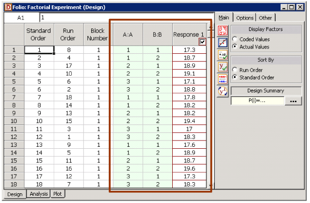
Consider an experiment to investigate the effect of speed and type of fuel additive used on the mileage of a sports utility vehicle. Three speeds and two types of fuel additives are investigated. Each of the treatment combinations are replicated three times. The mileage values observed are displayed in the fifth table.
The experimental design for the data in the fifth table is shown in the figure below. In the figure, the factor Speed is represented as factor [math]\displaystyle{ A\,\! }[/math] and the factor Fuel Additive is represented as factor [math]\displaystyle{ B\,\! }[/math]. The experimenter would like to investigate if speed, fuel additive or the interaction between speed and fuel additive affects the mileage of the sports utility vehicle. In other words, the following hypotheses need to be tested:
- [math]\displaystyle{ \begin{align} & \begin{matrix} 1. & {} \\ \end{matrix}{{H}_{0}}:{{\tau }_{1}}={{\tau }_{2}}={{\tau }_{3}}=0\text{ (No main effect of factor }A\text{, speed)} \\ & \begin{matrix} {} & {} \\ \end{matrix}{{H}_{1}}:{{\tau }_{i}}\ne 0\text{ for at least one }i \\ & \begin{matrix} 2. & {} \\ \end{matrix}{{H}_{0}}:{{\delta }_{1}}={{\delta }_{2}}={{\delta }_{3}}=0\text{ (No main effect of factor }B\text{, fuel additive)} \\ & \begin{matrix} {} & {} \\ \end{matrix}{{H}_{1}}:{{\delta }_{j}}\ne 0\text{ for at least one }j \\ & \begin{matrix} 3. & {} \\ \end{matrix}{{H}_{0}}:{{(\tau \delta )}_{11}}={{(\tau \delta )}_{12}}=...={{(\tau \delta )}_{33}}=0\text{ (No interaction }AB\text{)} \\ & \begin{matrix} {} & {} \\ \end{matrix}{{H}_{1}}:{{(\tau \delta )}_{ij}}\ne 0\text{ for at least one }ij \end{align}\,\! }[/math]
The test statistics for the three tests are:
- 1.[math]\displaystyle{ {{({{F}_{0}})}_{A}}=\frac{M{{S}_{A}}}{M{{S}_{E}}}\,\! }[/math]
- where [math]\displaystyle{ M{{S}_{A}}\,\! }[/math] is the mean square for factor [math]\displaystyle{ A\,\! }[/math] and [math]\displaystyle{ M{{S}_{E}}\,\! }[/math] is the error mean square
- 1.[math]\displaystyle{ {{({{F}_{0}})}_{A}}=\frac{M{{S}_{A}}}{M{{S}_{E}}}\,\! }[/math]
- 2.[math]\displaystyle{ {{({{F}_{0}})}_{B}}=\frac{M{{S}_{B}}}{M{{S}_{E}}}\,\! }[/math]
- where [math]\displaystyle{ M{{S}_{B}}\,\! }[/math] is the mean square for factor [math]\displaystyle{ B\,\! }[/math] and [math]\displaystyle{ M{{S}_{E}}\,\! }[/math] is the error mean square
- 2.[math]\displaystyle{ {{({{F}_{0}})}_{B}}=\frac{M{{S}_{B}}}{M{{S}_{E}}}\,\! }[/math]
- 3.[math]\displaystyle{ {{({{F}_{0}})}_{AB}}=\frac{M{{S}_{AB}}}{M{{S}_{E}}}\,\! }[/math]
- where [math]\displaystyle{ M{{S}_{AB}}\,\! }[/math] is the mean square for interaction [math]\displaystyle{ AB\,\! }[/math] and [math]\displaystyle{ M{{S}_{E}}\,\! }[/math] is the error mean square
- 3.[math]\displaystyle{ {{({{F}_{0}})}_{AB}}=\frac{M{{S}_{AB}}}{M{{S}_{E}}}\,\! }[/math]
The ANOVA model for this experiment can be written as:
- [math]\displaystyle{ {{Y}_{ijk}}=\mu +{{\tau }_{i}}+{{\delta }_{j}}+{{(\tau \delta )}_{ij}}+{{\epsilon }_{ijk}}\,\! }[/math]
where [math]\displaystyle{ {{\tau }_{i}}\,\! }[/math] represents the [math]\displaystyle{ i\,\! }[/math]th treatment of factor [math]\displaystyle{ A\,\! }[/math] (speed) with [math]\displaystyle{ i\,\! }[/math] =1, 2, 3; [math]\displaystyle{ {{\delta }_{j}}\,\! }[/math] represents the [math]\displaystyle{ j\,\! }[/math]th treatment of factor [math]\displaystyle{ B\,\! }[/math] (fuel additive) with [math]\displaystyle{ j\,\! }[/math] =1, 2; and [math]\displaystyle{ {{(\tau \delta )}_{ij}}\,\! }[/math] represents the interaction effect. In order to calculate the test statistics, it is convenient to express the ANOVA model of the equation given above in the form [math]\displaystyle{ y=X\beta +\epsilon \,\! }[/math]. This can be done as explained next.
Expression of the ANOVA Model as [math]\displaystyle{ y=X\beta +\epsilon \,\! }[/math]
Since the effects [math]\displaystyle{ {{\tau }_{i}}\,\! }[/math], [math]\displaystyle{ {{\delta }_{j}}\,\! }[/math] and [math]\displaystyle{ {{(\tau \delta )}_{ij}}\,\! }[/math] represent deviations from the overall mean, the following constraints exist. Constraints on [math]\displaystyle{ {{\tau }_{i}}\,\! }[/math] are:
- [math]\displaystyle{ \begin{align} \underset{i=1}{\overset{3}{\mathop \sum }}\,{{\tau }_{i}}= & 0 \\ \text{or }{{\tau }_{1}}+{{\tau }_{2}}+{{\tau }_{3}}= & 0 \end{align}\,\! }[/math]
Therefore, only two of the [math]\displaystyle{ {{\tau }_{i}}\,\! }[/math] effects are independent. Assuming that [math]\displaystyle{ {{\tau }_{1}}\,\! }[/math] and [math]\displaystyle{ {{\tau }_{2}}\,\! }[/math] are independent, [math]\displaystyle{ {{\tau }_{3}}=-({{\tau }_{1}}+{{\tau }_{2}})\,\! }[/math]. (The null hypothesis to test the significance of factor [math]\displaystyle{ A\,\! }[/math] can be rewritten using only the independent effects as [math]\displaystyle{ {{H}_{0}}:{{\tau }_{1}}={{\tau }_{2}}=0\,\! }[/math].) DOE++ displays only the independent effects because only these effects are important to the analysis. The independent effects, [math]\displaystyle{ {{\tau }_{1}}\,\! }[/math] and [math]\displaystyle{ {{\tau }_{2}}\,\! }[/math], are displayed as A[1] and A[2] respectively because these are the effects associated with factor [math]\displaystyle{ A\,\! }[/math] (speed).
Constraints on [math]\displaystyle{ {{\delta }_{j}}\,\! }[/math] are:
- [math]\displaystyle{ \begin{align} \underset{j=1}{\overset{2}{\mathop \sum }}\,{{\delta }_{j}}= & 0 \\ \text{or }{{\delta }_{1}}+{{\delta }_{2}}= & 0 \end{align}\,\! }[/math]
Therefore, only one of the [math]\displaystyle{ {{\delta }_{j}}\,\! }[/math] effects are independent. Assuming that [math]\displaystyle{ {{\delta }_{1}}\,\! }[/math] is independent, [math]\displaystyle{ {{\delta }_{2}}=-{{\delta }_{1}}\,\! }[/math]. (The null hypothesis to test the significance of factor [math]\displaystyle{ B\,\! }[/math] can be rewritten using only the independent effect as [math]\displaystyle{ {{H}_{0}}:{{\delta }_{1}}=0\,\! }[/math].) The independent effect [math]\displaystyle{ {{\delta }_{1}}\,\! }[/math] is displayed as B:B in DOE++.
Constraints on [math]\displaystyle{ {{(\tau \delta )}_{ij}}\,\! }[/math] are:
- [math]\displaystyle{ \begin{align} \underset{i=1}{\overset{3}{\mathop \sum }}\,{{(\tau \delta )}_{ij}}= & 0 \\ \text{and }\underset{j=1}{\overset{2}{\mathop \sum }}\,{{(\tau \delta )}_{ij}}= & 0 \\ \text{or }{{(\tau \delta )}_{11}}+{{(\tau \delta )}_{21}}+{{(\tau \delta )}_{31}}= & 0 \\ {{(\tau \delta )}_{12}}+{{(\tau \delta )}_{22}}+{{(\tau \delta )}_{32}}= & 0 \\ \text{and }{{(\tau \delta )}_{11}}+{{(\tau \delta )}_{12}}= & 0 \\ {{(\tau \delta )}_{21}}+{{(\tau \delta )}_{22}}= & 0 \\ {{(\tau \delta )}_{31}}+{{(\tau \delta )}_{32}}= & 0 \end{align}\,\! }[/math]
The last five equations given above represent four constraints, as only four of these five equations are independent. Therefore, only two out of the six [math]\displaystyle{ {{(\tau \delta )}_{ij}}\,\! }[/math] effects are independent. Assuming that [math]\displaystyle{ {{(\tau \delta )}_{11}}\,\! }[/math] and [math]\displaystyle{ {{(\tau \delta )}_{21}}\,\! }[/math] are independent, the other four effects can be expressed in terms of these effects. (The null hypothesis to test the significance of interaction [math]\displaystyle{ AB\,\! }[/math] can be rewritten using only the independent effects as [math]\displaystyle{ {{H}_{0}}:{{(\tau \delta )}_{11}}={{(\tau \delta )}_{21}}=0\,\! }[/math].) The effects [math]\displaystyle{ {{(\tau \delta )}_{11}}\,\! }[/math] and [math]\displaystyle{ {{(\tau \delta )}_{21}}\,\! }[/math] are displayed as A[1]B and A[2]B respectively in DOE++.
The regression version of the ANOVA model can be obtained using indicator variables, similar to the case of the single factor experiment in Fitting ANOVA Models. Since factor [math]\displaystyle{ A\,\! }[/math] has three levels, two indicator variables, [math]\displaystyle{ {{x}_{1}}\,\! }[/math] and [math]\displaystyle{ {{x}_{2}}\,\! }[/math], are required which need to be coded as shown next:
- [math]\displaystyle{ \begin{align} \text{Treatment Effect }{{\tau }_{1}}: & {{x}_{1}}=1,\text{ }{{x}_{2}}=0 \\ \text{Treatment Effect }{{\tau }_{2}}: & {{x}_{1}}=0,\text{ }{{x}_{2}}=1\text{ } \\ \text{Treatment Effect }{{\tau }_{3}}: & {{x}_{1}}=-1,\text{ }{{x}_{2}}=-1\text{ } \end{align}\,\! }[/math]
Factor [math]\displaystyle{ B\,\! }[/math] has two levels and can be represented using one indicator variable, [math]\displaystyle{ {{x}_{3}}\,\! }[/math], as follows:
- [math]\displaystyle{ \begin{align} \text{Treatment Effect }{{\delta }_{1}}: & {{x}_{3}}=1 \\ \text{Treatment Effect }{{\delta }_{2}}: & {{x}_{3}}=-1 \end{align}\,\! }[/math]
The [math]\displaystyle{ AB\,\! }[/math] interaction will be represented by all possible terms resulting from the product of the indicator variables representing factors [math]\displaystyle{ A\,\! }[/math] and [math]\displaystyle{ B\,\! }[/math]. There are two such terms here - [math]\displaystyle{ {{x}_{1}}{{x}_{3}}\,\! }[/math] and [math]\displaystyle{ {{x}_{2}}{{x}_{3}}\,\! }[/math]. The regression version of the ANOVA model can finally be obtained as:
- [math]\displaystyle{ Y=\mu +{{\tau }_{1}}\cdot {{x}_{1}}+{{\tau }_{2}}\cdot {{x}_{2}}+{{\delta }_{1}}\cdot {{x}_{3}}+{{(\tau \delta )}_{11}}\cdot {{x}_{1}}{{x}_{3}}+{{(\tau \delta )}_{21}}\cdot {{x}_{2}}{{x}_{3}}+\epsilon \,\! }[/math]
In matrix notation this model can be expressed as:
- [math]\displaystyle{ y=X\beta +\epsilon \,\! }[/math]
- where:
- [math]\displaystyle{ y=\left[ \begin{matrix} {{Y}_{111}} \\ {{Y}_{211}} \\ {{Y}_{311}} \\ {{Y}_{121}} \\ {{Y}_{221}} \\ {{Y}_{321}} \\ {{Y}_{112}} \\ {{Y}_{212}} \\ . \\ . \\ {{Y}_{323}} \\ \end{matrix} \right]=X\beta +\epsilon =\left[ \begin{matrix} 1 & 1 & 0 & 1 & 1 & 0 \\ 1 & 0 & 1 & 1 & 0 & 1 \\ 1 & -1 & -1 & 1 & -1 & -1 \\ 1 & 1 & 0 & -1 & -1 & 0 \\ 1 & 0 & 1 & -1 & 0 & -1 \\ 1 & -1 & -1 & -1 & 1 & 1 \\ 1 & 1 & 0 & 1 & 1 & 0 \\ 1 & 0 & 1 & 1 & 0 & 1 \\ . & . & . & . & . & . \\ . & . & . & . & . & . \\ 1 & -1 & -1 & -1 & 1 & 1 \\ \end{matrix} \right]\left[ \begin{matrix} \mu \\ {{\tau }_{1}} \\ {{\tau }_{2}} \\ {{\delta }_{1}} \\ {{(\tau \delta )}_{11}} \\ {{(\tau \delta )}_{21}} \\ \end{matrix} \right]+\left[ \begin{matrix} {{\epsilon }_{111}} \\ {{\epsilon }_{211}} \\ {{\epsilon }_{311}} \\ {{\epsilon }_{121}} \\ {{\epsilon }_{221}} \\ {{\epsilon }_{321}} \\ {{\epsilon }_{112}} \\ {{\epsilon }_{212}} \\ . \\ . \\ {{\epsilon }_{323}} \\ \end{matrix} \right]\,\! }[/math]
The vector [math]\displaystyle{ y\,\! }[/math] can be substituted with the response values from the fifth table to get:
- [math]\displaystyle{ y=\left[ \begin{matrix} {{Y}_{111}} \\ {{Y}_{211}} \\ {{Y}_{311}} \\ {{Y}_{121}} \\ {{Y}_{221}} \\ {{Y}_{321}} \\ {{Y}_{112}} \\ {{Y}_{212}} \\ . \\ . \\ {{Y}_{323}} \\ \end{matrix} \right]=\left[ \begin{matrix} 17.3 \\ 18.9 \\ 17.1 \\ 18.7 \\ 19.1 \\ 18.8 \\ 17.8 \\ 18.2 \\ . \\ . \\ 18.3 \\ \end{matrix} \right]\,\! }[/math]
Knowing [math]\displaystyle{ y\,\! }[/math], [math]\displaystyle{ X\,\! }[/math] and [math]\displaystyle{ \beta \,\! }[/math], the sum of squares for the ANOVA model and the extra sum of squares for each of the factors can be calculated. These are used to calculate the mean squares that are used to obtain the test statistics.
Calculation of Sum of Squares for the Model
The model sum of squares, [math]\displaystyle{ S{{S}_{TR}}\,\! }[/math], for the regression version of the ANOVA model can be obtained as:
- [math]\displaystyle{ \begin{align} S{{S}_{TR}}= & {{y}^{\prime }}[H-(\frac{1}{{{n}_{a}}\cdot {{n}_{b}}\cdot m})J]y \\ = & {{y}^{\prime }}[H-(\frac{1}{18})J]y \\ = & 9.7311 \end{align}\,\! }[/math]
where [math]\displaystyle{ H\,\! }[/math] is the hat matrix and [math]\displaystyle{ J\,\! }[/math] is the matrix of ones. Since five effect terms ([math]\displaystyle{ {{\tau }_{1}}\,\! }[/math], [math]\displaystyle{ {{\tau }_{2}}\,\! }[/math], [math]\displaystyle{ {{\delta }_{1}}\,\! }[/math], [math]\displaystyle{ {{(\tau \delta )}_{11}}\,\! }[/math] and [math]\displaystyle{ {{(\tau \delta )}_{21}}\,\! }[/math]) are used in the model, the number of degrees of freedom associated with [math]\displaystyle{ S{{S}_{TR}}\,\! }[/math] is five ([math]\displaystyle{ dof(S{{S}_{TR}})=5\,\! }[/math]).
The total sum of squares, [math]\displaystyle{ S{{S}_{T}}\,\! }[/math], can be calculated as:
- [math]\displaystyle{ \begin{align} S{{S}_{T}}= & {{y}^{\prime }}[I-(\frac{1}{{{n}_{a}}\cdot {{n}_{b}}\cdot m})J]y \\ = & {{y}^{\prime }}[I-(\frac{1}{18})J]y \\ = & 10.7178 \end{align}\,\! }[/math]
Since there are 18 observed response values, the number of degrees of freedom associated with the total sum of squares is 17 ([math]\displaystyle{ dof(S{{S}_{T}})=17\,\! }[/math]). The error sum of squares can now be obtained:
- [math]\displaystyle{ \begin{align} S{{S}_{E}}= & S{{S}_{T}}-S{{S}_{TR}} \\ = & 10.7178-9.7311 \\ = & 0.9867 \end{align}\,\! }[/math]
Since there are three replicates of the full factorial experiment, all of the error sum of squares is pure error. (This can also be seen from the preceding figure, where each treatment combination of the full factorial design is repeated three times.) The number of degrees of freedom associated with the error sum of squares is:
- [math]\displaystyle{ \begin{align} dof(S{{S}_{E}})= & dof(S{{S}_{T}})-dof(S{{S}_{TR}}) \\ = & 17-5 \\ = & 12 \end{align}\,\! }[/math]
Calculation of Extra Sum of Squares for the Factors
The sequential sum of squares for factor [math]\displaystyle{ A\,\! }[/math] can be calculated as:
- [math]\displaystyle{ \begin{align} S{{S}_{A}}= & S{{S}_{TR}}(\mu ,{{\tau }_{1}},{{\tau }_{2}})-S{{S}_{TR}}(\mu ) \\ = & {{y}^{\prime }}[{{H}_{\mu ,{{\tau }_{1}},{{\tau }_{2}}}}-(\frac{1}{18})J]y-0 \end{align}\,\! }[/math]
where [math]\displaystyle{ {{H}_{\mu ,{{\tau }_{1}},{{\tau }_{2}}}}={{X}_{\mu ,{{\tau }_{1}},{{\tau }_{2}}}}{{(X_{\mu ,{{\tau }_{1}},{{\tau }_{2}}}^{\prime }{{X}_{\mu ,{{\tau }_{1}},{{\tau }_{2}}}})}^{-1}}X_{\mu ,{{\tau }_{1}},{{\tau }_{2}}}^{\prime }\,\! }[/math] and [math]\displaystyle{ {{X}_{\mu ,{{\tau }_{1}},{{\tau }_{2}}}}\,\! }[/math] is the matrix containing only the first three columns of the [math]\displaystyle{ X\,\! }[/math] matrix. Thus:
- [math]\displaystyle{ \begin{align} S{{S}_{A}}= & {{y}^{\prime }}[{{H}_{\mu ,{{\tau }_{1}},{{\tau }_{2}}}}-(\frac{1}{18})J]y-0 \\ = & 4.5811-0 \\ = & 4.5811 \end{align}\,\! }[/math]
Since there are two independent effects ([math]\displaystyle{ {{\tau }_{1}}\,\! }[/math], [math]\displaystyle{ {{\tau }_{2}}\,\! }[/math]) for factor [math]\displaystyle{ A\,\! }[/math], the degrees of freedom associated with [math]\displaystyle{ S{{S}_{A}}\,\! }[/math] are two ([math]\displaystyle{ dof(S{{S}_{A}})=2\,\! }[/math]).
Similarly, the sum of squares for factor [math]\displaystyle{ B\,\! }[/math] can be calculated as:
- [math]\displaystyle{ \begin{align} S{{S}_{B}}= & S{{S}_{TR}}(\mu ,{{\tau }_{1}},{{\tau }_{2}},{{\delta }_{1}})-S{{S}_{TR}}(\mu ,{{\tau }_{1}},{{\tau }_{2}}) \\ = & {{y}^{\prime }}[{{H}_{\mu ,{{\tau }_{1}},{{\tau }_{2}},{{\delta }_{1}}}}-(\frac{1}{18})J]y-{{y}^{\prime }}[{{H}_{\mu ,{{\tau }_{1}},{{\tau }_{2}}}}-(\frac{1}{18})J]y \\ = & 9.4900-4.5811 \\ = & 4.9089 \end{align}\,\! }[/math]
Since there is one independent effect, [math]\displaystyle{ {{\delta }_{1}}\,\! }[/math], for factor [math]\displaystyle{ B\,\! }[/math], the number of degrees of freedom associated with [math]\displaystyle{ S{{S}_{B}}\,\! }[/math] is one ([math]\displaystyle{ dof(S{{S}_{B}})=1\,\! }[/math]).
The sum of squares for the interaction [math]\displaystyle{ AB\,\! }[/math] is:
- [math]\displaystyle{ \begin{align} S{{S}_{AB}}= & S{{S}_{TR}}(\mu ,{{\tau }_{1}},{{\tau }_{2}},{{\delta }_{1}},{{(\tau \delta )}_{11}},{{(\tau \delta )}_{21}})-S{{S}_{TR}}(\mu ,{{\tau }_{1}},{{\tau }_{2}},{{\delta }_{1}}) \\ = & S{{S}_{TR}}-S{{S}_{TR}}(\mu ,{{\tau }_{1}},{{\tau }_{2}},{{\delta }_{1}}) \\ = & 9.7311-9.4900 \\ = & 0.2411 \end{align}\,\! }[/math]
Since there are two independent interaction effects, [math]\displaystyle{ {{(\tau \delta )}_{11}}\,\! }[/math] and [math]\displaystyle{ {{(\tau \delta )}_{21}}\,\! }[/math], the number of degrees of freedom associated with [math]\displaystyle{ S{{S}_{AB}}\,\! }[/math] is two ([math]\displaystyle{ dof(S{{S}_{AB}})=2\,\! }[/math]).
Calculation of the Test Statistics
Knowing the sum of squares, the test statistic for each of the factors can be calculated. Analyzing the interaction first, the test statistic for interaction [math]\displaystyle{ AB\,\! }[/math] is:
- [math]\displaystyle{ \begin{align} {{({{f}_{0}})}_{AB}}= & \frac{M{{S}_{AB}}}{M{{S}_{E}}} \\ = & \frac{0.2411/2}{0.9867/12} \\ = & 1.47 \end{align}\,\! }[/math]
The [math]\displaystyle{ p\,\! }[/math] value corresponding to this statistic, based on the [math]\displaystyle{ F\,\! }[/math] distribution with 2 degrees of freedom in the numerator and 12 degrees of freedom in the denominator, is:
- [math]\displaystyle{ \begin{align} p\text{ }value= & 1-P(F\le {{({{f}_{0}})}_{AB}}) \\ = & 1-0.7307 \\ = & 0.2693 \end{align}\,\! }[/math]
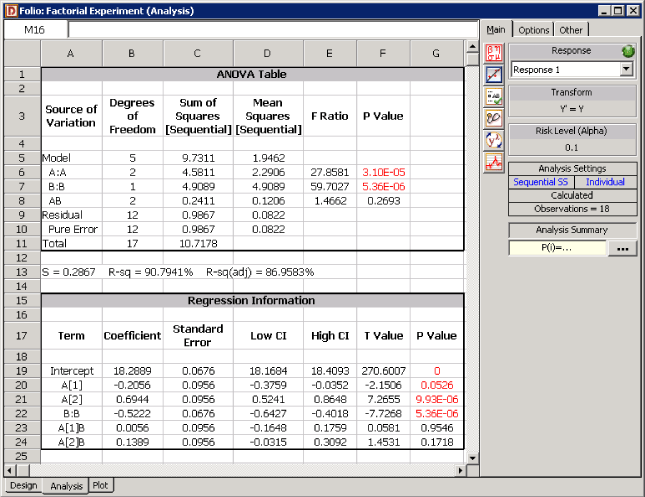
Assuming that the desired significance level is 0.1, since [math]\displaystyle{ p\,\! }[/math] value > 0.1, we fail to reject [math]\displaystyle{ {{H}_{0}}:{{(\tau \delta )}_{ij}}=0\,\! }[/math] and conclude that the interaction between speed and fuel additive does not significantly affect the mileage of the sports utility vehicle. DOE++ displays this result in the ANOVA table, as shown in the following figure. In the absence of the interaction, the analysis of main effects becomes important.
The test statistic for factor [math]\displaystyle{ A\,\! }[/math] is:
- [math]\displaystyle{ \begin{align} {{({{f}_{0}})}_{A}}= & \frac{M{{S}_{A}}}{M{{S}_{E}}} \\ = & \frac{S{{S}_{A}}/dof(S{{S}_{A}})}{S{{S}_{E}}/dof(S{{S}_{E}})} \\ = & \frac{4.5811/2}{0.9867/12} \\ = & 27.86 \end{align}\,\! }[/math]
The [math]\displaystyle{ p\,\! }[/math] value corresponding to this statistic based on the [math]\displaystyle{ F\,\! }[/math] distribution with 2 degrees of freedom in the numerator and 12 degrees of freedom in the denominator is:
- [math]\displaystyle{ \begin{align} p\text{ }value= & 1-P(F\le {{({{f}_{0}})}_{A}}) \\ = & 1-0.99997 \\ = & 0.00003 \end{align}\,\! }[/math]
Since [math]\displaystyle{ p\,\! }[/math] value < 0.1, [math]\displaystyle{ {{H}_{0}}:{{\tau }_{i}}=0\,\! }[/math] is rejected and it is concluded that factor [math]\displaystyle{ A\,\! }[/math] (or speed) has a significant effect on the mileage.
The test statistic for factor [math]\displaystyle{ B\,\! }[/math] is:
- [math]\displaystyle{ \begin{align} {{({{f}_{0}})}_{B}}= & \frac{M{{S}_{B}}}{M{{S}_{E}}} \\ = & \frac{4.9089/1}{0.9867/12} \\ = & 59.7 \end{align}\,\! }[/math]
The [math]\displaystyle{ p\,\! }[/math] value corresponding to this statistic based on the [math]\displaystyle{ F\,\! }[/math] distribution with 2 degrees of freedom in the numerator and 12 degrees of freedom in the denominator is:
- [math]\displaystyle{ \begin{align} p\text{ }value= & 1-P(F\le {{({{f}_{0}})}_{B}}) \\ = & 1-0.999995 \\ = & 0.000005 \end{align}\,\! }[/math]
Since [math]\displaystyle{ p\,\! }[/math] value < 0.1, [math]\displaystyle{ {{H}_{0}}:{{\delta }_{j}}=0\,\! }[/math] is rejected and it is concluded that factor [math]\displaystyle{ B\,\! }[/math] (or fuel additive type) has a significant effect on the mileage.
Therefore, it can be concluded that speed and fuel additive type affect the mileage of the vehicle significantly. The results are displayed in the ANOVA table of the following figure.
Calculation of Effect Coefficients
Results for the effect coefficients of the model of the regression version of the ANOVA model are displayed in the Regression Information table in the following figure. Calculations of the results in this table are discussed next. The effect coefficients can be calculated as follows:
- [math]\displaystyle{ \begin{align} \hat{\beta }= & {{({{X}^{\prime }}X)}^{-1}}{{X}^{\prime }}y \\ = & \left[ \begin{matrix} 18.2889 \\ -0.2056 \\ 0.6944 \\ -0.5222 \\ 0.0056 \\ 0.1389 \\ \end{matrix} \right] \end{align}\,\! }[/math]
Therefore, [math]\displaystyle{ \hat{\mu }=18.2889\,\! }[/math], [math]\displaystyle{ {{\hat{\tau }}_{1}}=-0.2056\,\! }[/math], [math]\displaystyle{ {{\hat{\tau }}_{2}}=0.6944\,\! }[/math] etc. As mentioned previously, these coefficients are displayed as Intercept, A[1] and A[2] respectively depending on the name of the factor used in the experimental design. The standard error for each of these estimates is obtained using the diagonal elements of the variance-covariance matrix [math]\displaystyle{ C\,\! }[/math].
- [math]\displaystyle{ \begin{align} C= & {{{\hat{\sigma }}}^{2}}{{({{X}^{\prime }}X)}^{-1}} \\ = & M{{S}_{E}}\cdot {{({{X}^{\prime }}X)}^{-1}} \\ = & \left[ \begin{matrix} 0.0046 & 0 & 0 & 0 & 0 & 0 \\ 0 & 0.0091 & -0.0046 & 0 & 0 & 0 \\ 0 & -0.0046 & 0.0091 & 0 & 0 & 0 \\ 0 & 0 & 0 & 0.0046 & 0 & 0 \\ 0 & 0 & 0 & 0 & 0.0091 & -0.0046 \\ 0 & 0 & 0 & 0 & -0.0046 & 0.0091 \\ \end{matrix} \right] \end{align}\,\! }[/math]
For example, the standard error for [math]\displaystyle{ {{\hat{\tau }}_{1}}\,\! }[/math] is:
- [math]\displaystyle{ \begin{align} se({{{\hat{\tau }}}_{1}})= & \sqrt{{{C}_{22}}} \\ = & \sqrt{0.0091} \\ = & 0.0956 \end{align}\,\! }[/math]
Then the [math]\displaystyle{ t\,\! }[/math] statistic for [math]\displaystyle{ {{\hat{\tau }}_{1}}\,\! }[/math] can be obtained as:
- [math]\displaystyle{ \begin{align} {{t}_{0}}= & \frac{{{{\hat{\tau }}}_{1}}}{se({{{\hat{\tau }}}_{1}})} \\ = & \frac{-0.2056}{0.0956} \\ = & -2.1506 \end{align}\,\! }[/math]
The [math]\displaystyle{ p\,\! }[/math] value corresponding to this statistic is:
Confidence intervals on [math]\displaystyle{ {{\tau }_{1}}\,\! }[/math] can also be calculated. The 90% limits on [math]\displaystyle{ {{\tau }_{1}}\,\! }[/math] are:
- [math]\displaystyle{ \begin{align} = & {{{\hat{\tau }}}_{1}}\pm {{t}_{\alpha /2,n-(k+1)}}\sqrt{{{C}_{22}}} \\ = & {{\tau }_{1}}\pm {{t}_{0.05,12}}\sqrt{{{C}_{22}}} \\ = & -0.2056\pm 0.1704 \end{align}\,\! }[/math]
Thus, the 90% limits on [math]\displaystyle{ {{\tau }_{1}}\,\! }[/math] are [math]\displaystyle{ -0.3760\,\! }[/math] and [math]\displaystyle{ -0.0352\,\! }[/math] respectively. Results for other coefficients are obtained in a similar manner.
Least Squares Means
The estimated mean response corresponding to the [math]\displaystyle{ i\,\! }[/math]th level of any factor is obtained using the adjusted estimated mean which is also called the least squares mean. For example, the mean response corresponding to the first level of factor [math]\displaystyle{ A\,\! }[/math] is [math]\displaystyle{ \mu +{{\tau }_{1}}\,\! }[/math]. An estimate of this is [math]\displaystyle{ \hat{\mu }+{{\hat{\tau }}_{1}}\,\! }[/math] or ([math]\displaystyle{ 18.2889+(-0.2056)=18.0833\,\! }[/math]). Similarly, the estimated response at the third level of factor [math]\displaystyle{ A\,\! }[/math] is [math]\displaystyle{ \hat{\mu }+{{\hat{\tau }}_{3}}\,\! }[/math] or [math]\displaystyle{ \hat{\mu }+(-{{\hat{\tau }}_{1}}-{{\hat{\tau }}_{2}})\,\! }[/math] or ([math]\displaystyle{ 18.2889+(0.2056-0.6944)=17.8001\,\! }[/math]).
Residual Analysis
As in the case of single factor experiments, plots of residuals can also be used to check for model adequacy in factorial experiments. Box-Cox transformations are also available in DOE++ for factorial experiments.

