Likelihood Ratio Test Example: Difference between revisions
No edit summary |
No edit summary |
||
| Line 35: | Line 35: | ||
The assumption of a common <math>\beta \,\!</math> across the different stress levels can be visually assessed by using a probability plot. As you can see in the following plot, the plotted data from the different stress levels seem to be fairly parallel. | The assumption of a common <math>\beta \,\!</math> across the different stress levels can be visually assessed by using a probability plot. As you can see in the following plot, the plotted data from the different stress levels seem to be fairly parallel. | ||
[[Image:3linedplot.png|center| | [[Image:3linedplot.png|center|600px|Probability plot of the three test stress levels.]] | ||
A better assessment can be made with the LR test, which can be performed using the Likelihood Ratio Test tool in ALTA. For example, in the following figure, the <math>\beta s\,\!</math> are compared for equality at the 10% level. | A better assessment can be made with the LR test, which can be performed using the Likelihood Ratio Test tool in ALTA. For example, in the following figure, the <math>\beta s\,\!</math> are compared for equality at the 10% level. | ||
Revision as of 17:18, 21 December 2015
New format available! This reference is now available in a new format that offers faster page load, improved display for calculations and images and more targeted search.
As of January 2024, this Reliawiki page will not continue to be updated. Please update all links and bookmarks to the latest references at ALTA examples and ALTA reference examples.
This example appears in the Accelerated Life Testing Data Analysis Reference book.
Consider the following times-to-failure data at three different stress levels.
| Stress | 406 K | 416 K | 426 K |
|---|---|---|---|
| Time Failed (hrs) | 248 | 164 | 92 |
| 456 | 176 | 105 | |
| 528 | 289 | 155 | |
| 731 | 319 | 184 | |
| 813 | 340 | 219 | |
| 543 | 235 |
The data set was analyzed using an Arrhenius-Weibull model. The analysis yields:
- [math]\displaystyle{ \widehat{\beta }=\ 2.965820\,\! }[/math]
- [math]\displaystyle{ \widehat{B}=\ 10,679.567542\,\! }[/math]
- [math]\displaystyle{ \widehat{C}=\ 2.396615\cdot {{10}^{-9}}\,\! }[/math]
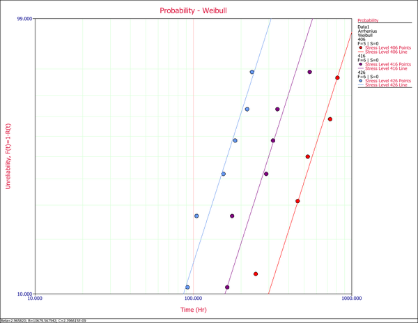
The assumption of a common [math]\displaystyle{ \beta \,\! }[/math] across the different stress levels can be visually assessed by using a probability plot. As you can see in the following plot, the plotted data from the different stress levels seem to be fairly parallel.
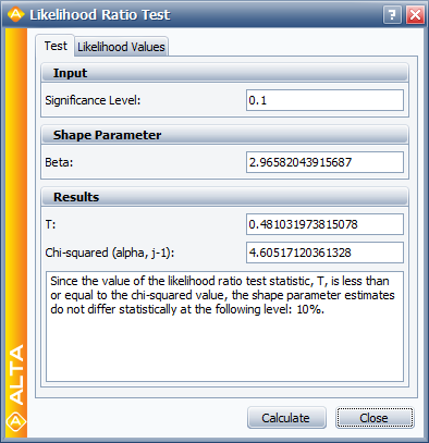
A better assessment can be made with the LR test, which can be performed using the Likelihood Ratio Test tool in ALTA. For example, in the following figure, the [math]\displaystyle{ \beta s\,\! }[/math] are compared for equality at the 10% level.
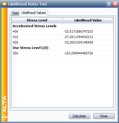
The LR test statistic, [math]\displaystyle{ T\,\! }[/math], is calculated to be 0.481. Therefore, [math]\displaystyle{ T=0.481\le 4.605={{\chi }^{2}}(0.9;2),\,\! }[/math] the [math]\displaystyle{ {\beta }'\,\! }[/math] s do not differ significantly at the 10% level. The individual likelihood values for each of the test stresses are shown next.


