Multiple Linear Regression Analysis

Introduction

This chapter expands on the analysis of simple linear regression models and discusses the analysis of multiple linear regression models. A major portion of the results displayed in DOE++ are explained in this chapter because these results are associated with multiple linear regression. One of the applications of multiple linear regression models is Response Surface Methodology (RSM). RSM is a method used to locate the optimum value of the response and is one of the final stages of experimentation. It is discussed in Chapter 9. Towards the end of this chapter, the concept of using indicator variables in regression models is explained. Indicator variables are used to represent qualitative factors in regression models. The concept of using indicator variables is important to gain an understanding of ANOVA models, which are the models used to analyze data obtained from experiments. These models can be thought of as first order multiple linear regression models where all the factors are treated as qualitative factors. ANOVA models are discussed in Chapter 6.

Multiple Linear Regression Model

A linear regression model that contains more than one predictor variable is called a multiple linear regression model. The following model is a multiple linear regression model with two predictor variables, [math]\displaystyle{ {{x}_{1}} }[/math] and [math]\displaystyle{ {{x}_{2}} }[/math] .

[math]\displaystyle{ Y={{\beta }_{0}}+{{\beta }_{1}}{{x}_{1}}+{{\beta }_{2}}{{x}_{2}}+\epsilon }[/math]

The model is linear because it is linear in the parameters [math]\displaystyle{ {{\beta }_{0}} }[/math] , [math]\displaystyle{ {{\beta }_{1}} }[/math] and [math]\displaystyle{ {{\beta }_{2}} }[/math] . The model describes a plane in the three dimensional space of [math]\displaystyle{ Y }[/math] , [math]\displaystyle{ {{x}_{1}} }[/math] and [math]\displaystyle{ {{x}_{2}} }[/math] . The parameter [math]\displaystyle{ {{\beta }_{0}} }[/math] is the intercept of this plane. Parameters [math]\displaystyle{ {{\beta }_{1}} }[/math] and [math]\displaystyle{ {{\beta }_{2}} }[/math] are referred to as partial regression coefficients. Parameter [math]\displaystyle{ {{\beta }_{1}} }[/math] represents the change in the mean response corresponding to a unit change in [math]\displaystyle{ {{x}_{1}} }[/math] when [math]\displaystyle{ {{x}_{2}} }[/math] is held constant. Parameter [math]\displaystyle{ {{\beta }_{2}} }[/math] represents the change in the mean response corresponding to a unit change in [math]\displaystyle{ {{x}_{2}} }[/math] when [math]\displaystyle{ {{x}_{1}} }[/math] is held constant. Consider the following example of a multiple linear regression model with two predictor variables, [math]\displaystyle{ {{x}_{1}} }[/math] and [math]\displaystyle{ {{x}_{2}} }[/math] :

[math]\displaystyle{ Y=30+5{{x}_{1}}+7{{x}_{2}}+\epsilon }[/math]

This regression model is a first order multiple linear regression model. This is because the maximum power of the variables in the model is one. The regression plane corresponding to this model is shown in Figure TrueRegrPlane. Also shown is an observed data point and the corresponding random error, [math]\displaystyle{ \epsilon }[/math] . The true regression model is usually never known (and therefore the values of the random error terms corresponding to observed data points remain unknown). However, the regression model can be estimated by calculating the parameters of the model for an observed data set. This is explained in Section 5.MatrixApproach.

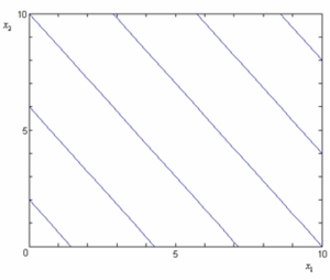
Figure ContourPlot1 shows the contour plot for the regression model of Eqn. (FirstOrderModelExample). The contour plot shows lines of constant mean response values as a function of [math]\displaystyle{ {{x}_{1}} }[/math] and [math]\displaystyle{ {{x}_{2}} }[/math] . The contour lines for the given regression model are straight lines as seen on the plot. Straight contour lines result for first order regression models with no interaction terms.

A linear regression model may also take the following form:

[math]\displaystyle{ Y={{\beta }_{0}}+{{\beta }_{1}}{{x}_{1}}+{{\beta }_{2}}{{x}_{2}}+{{\beta }_{12}}{{x}_{1}}{{x}_{2}}+\epsilon }[/math]

Regression plane for the model [math]\displaystyle{ Y=30+5 x_1+7 x_2+\epsilon }[/math]

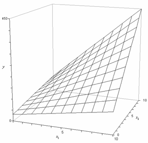
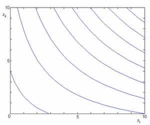
A cross-product term, [math]\displaystyle{ {{x}_{1}}{{x}_{2}} }[/math] , is included in the model. This term represents an interaction effect between the two variables [math]\displaystyle{ {{x}_{1}} }[/math] and [math]\displaystyle{ {{x}_{2}} }[/math] . Interaction means that the effect produced by a change in the predictor variable on the response depends on the level of the other predictor variable(s). As an example of a linear regression model with interaction, consider the model given by the equation [math]\displaystyle{ Y=30+5{{x}_{1}}+7{{x}_{2}}+3{{x}_{1}}{{x}_{2}}+\epsilon }[/math] . The regression plane and contour plot for this model are shown in Figures RegrPlaneWInteraction and ContourPlotWInteraction, respectively.

Countour plot for the model [math]\displaystyle{ Y=30+5 x_1+7 x_2+\epsilon }[/math]

Now consider the regression model shown next:

[math]\displaystyle{ Y={{\beta }_{0}}+{{\beta }_{1}}{{x}_{1}}+{{\beta }_{2}}x_{1}^{2}+{{\beta }_{3}}x_{1}^{3}+\epsilon }[/math]

This model is also a linear regression model and is referred to as a polynomial regression model. Polynomial regression models contain squared and higher order terms of the predictor variables making the response surface curvilinear. As an example of a polynomial regression model with an interaction term consider the following equation:

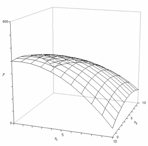
[math]\displaystyle{ Y=500+5{{x}_{1}}+7{{x}_{2}}-3x_{1}^{2}-5x_{2}^{2}+3{{x}_{1}}{{x}_{2}}+\epsilon }[/math]

Regression plane for the model [math]\displaystyle{ Y=30+5 x_1+7 x_2+3 x_1 x_2+\epsilon }[/math]

Countour plot for the model [math]\displaystyle{ Y=30+5 x_1+7 x_2+3 x_1 x_2+\epsilon }[/math]

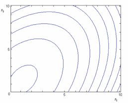
This model is a second order model because the maximum power of the terms in the model is two. The regression surface for this model is shown in Figure PolynomialRegrSurface. Such regression models are used in RSM to find the optimum value of the response, [math]\displaystyle{ Y }[/math] (for details see Chapter 9). Notice that, although the shape of the regression surface is curvilinear, the regression model of Eqn. (SecondOrderModelEx) is still linear because the model is linear in the parameters. The contour plot for this model is shown in Figure ContourPlotPolynomialRegr. All multiple linear regression models can be expressed in the following general form:

[math]\displaystyle{ Y={{\beta }_{0}}+{{\beta }_{1}}{{x}_{1}}+{{\beta }_{2}}{{x}_{2}}+...+{{\beta }_{k}}{{x}_{k}}+\epsilon }[/math]

where [math]\displaystyle{ k }[/math] denotes the number of terms in the model. For example, the model of Eqn. (SecondOrderModelEx) can be written in the general form using [math]\displaystyle{ {{x}_{3}}=x_{1}^{2} }[/math] , [math]\displaystyle{ {{x}_{4}}=x_{2}^{3} }[/math] and [math]\displaystyle{ {{x}_{5}}={{x}_{1}}{{x}_{2}} }[/math] as follows:

[math]\displaystyle{ Y=500+5{{x}_{1}}+7{{x}_{2}}-3{{x}_{3}}-5{{x}_{4}}+3{{x}_{5}}+\epsilon }[/math]

Estimating Regression Models Using Least Squares

Consider a multiple linear regression model with [math]\displaystyle{ k }[/math] predictor variables:

[math]\displaystyle{ Y={{\beta }_{0}}+{{\beta }_{1}}{{x}_{1}}+{{\beta }_{2}}{{x}_{2}}+...+{{\beta }_{k}}{{x}_{k}}+\epsilon }[/math]

Let each of the [math]\displaystyle{ k }[/math] predictor variables, [math]\displaystyle{ {{x}_{1}} }[/math] , [math]\displaystyle{ {{x}_{2}} }[/math] ... [math]\displaystyle{ {{x}_{k}} }[/math] , have [math]\displaystyle{ n }[/math] levels. Then [math]\displaystyle{ {{x}_{ij}} }[/math] represents the [math]\displaystyle{ i }[/math] th level of the [math]\displaystyle{ j }[/math] th predictor variable [math]\displaystyle{ {{x}_{j}} }[/math] . For example, [math]\displaystyle{ {{x}_{51}} }[/math] represents the fifth level of the first predictor variable [math]\displaystyle{ {{x}_{1}} }[/math] , while [math]\displaystyle{ {{x}_{19}} }[/math] represents the first level of the ninth predictor variable, [math]\displaystyle{ {{x}_{9}} }[/math] . Observations, [math]\displaystyle{ {{y}_{1}} }[/math] , [math]\displaystyle{ {{y}_{2}} }[/math] ... [math]\displaystyle{ {{y}_{n}} }[/math] , recorded for each of these [math]\displaystyle{ n }[/math] levels can be expressed in the following way:

[math]\displaystyle{ \begin{align} & {{y}_{1}}= & {{\beta }_{0}}+{{\beta }_{1}}{{x}_{11}}+{{\beta }_{2}}{{x}_{12}}+...+{{\beta }_{k}}{{x}_{1k}}+{{\epsilon }_{1}} \\ & {{y}_{2}}= & {{\beta }_{0}}+{{\beta }_{1}}{{x}_{21}}+{{\beta }_{2}}{{x}_{22}}+...+{{\beta }_{k}}{{x}_{2k}}+{{\epsilon }_{2}} \\ & & .. \\ & {{y}_{i}}= & {{\beta }_{0}}+{{\beta }_{1}}{{x}_{i1}}+{{\beta }_{2}}{{x}_{i2}}+...+{{\beta }_{k}}{{x}_{ik}}+{{\epsilon }_{i}} \\ & & .. \\ & {{y}_{n}}= & {{\beta }_{0}}+{{\beta }_{1}}{{x}_{n1}}+{{\beta }_{2}}{{x}_{n2}}+...+{{\beta }_{k}}{{x}_{nk}}+{{\epsilon }_{n}} \end{align} }[/math]

Regression surface for the model [math]\displaystyle{ 500+5 x_1+7 x_2-3 x_1^2-5 x_2^2+3 x_1 x_2+\epsilon }[/math].

Contour plot for the model [math]\displaystyle{ 500+5 x_1+7 x_2-3 x_1^2-5 x_2^2+3 x_1 x_2+\epsilon }[/math].

The system of [math]\displaystyle{ n }[/math] equations shown previously can be represented in matrix notation as follows:

[math]\displaystyle{ y=X\beta +\epsilon }[/math]

where

[math]\displaystyle{ y=\left[ \begin{matrix} {{y}_{1}} \\ {{y}_{2}} \\ . \\ . \\ . \\ {{y}_{n}} \\ \end{matrix} \right]\text{ }X=\left[ \begin{matrix} 1 & {{x}_{11}} & {{x}_{12}} & . & . & . & {{x}_{1n}} \\ 1 & {{x}_{21}} & {{x}_{22}} & . & . & . & {{x}_{2n}} \\ . & . & . & {} & {} & {} & . \\ . & . & . & {} & {} & {} & . \\ . & . & . & {} & {} & {} & . \\ 1 & {{x}_{n1}} & {{x}_{n2}} & . & . & . & {{x}_{nn}} \\ \end{matrix} \right] }[/math]

[math]\displaystyle{ \beta =\left[ \begin{matrix} {{\beta }_{0}} \\ {{\beta }_{1}} \\ . \\ . \\ . \\ {{\beta }_{n}} \\ \end{matrix} \right]\text{ and }\epsilon =\left[ \begin{matrix} {{\epsilon }_{1}} \\ {{\epsilon }_{2}} \\ . \\ . \\ . \\ {{\epsilon }_{n}} \\ \end{matrix} \right] }[/math]

The matrix [math]\displaystyle{ X }[/math] in Eqn. (TrueModelMatrixNotation) is referred to as the design matrix. It contains information about the levels of the predictor variables at which the observations are obtained. The vector [math]\displaystyle{ \beta }[/math] contains all the regression coefficients. To obtain the regression model, [math]\displaystyle{ \beta }[/math] should be known. [math]\displaystyle{ \beta }[/math] is estimated using least square estimates. The following equation is used:

[math]\displaystyle{ \hat{\beta }={{({{X}^{\prime }}X)}^{-1}}{{X}^{\prime }}y }[/math]

where [math]\displaystyle{ ^{\prime } }[/math] represents the transpose of the matrix while [math]\displaystyle{ ^{-1} }[/math] represents the matrix inverse. Knowing the estimates, [math]\displaystyle{ \hat{\beta } }[/math] , the multiple linear regression model can now be estimated as:

[math]\displaystyle{ \hat{y}=X\hat{\beta } }[/math]

The estimated regression model is also referred to as the fitted model. The observations, [math]\displaystyle{ {{y}_{i}} }[/math] , may be different from the fitted values [math]\displaystyle{ {{\hat{y}}_{i}} }[/math] obtained from this model. The difference between these two values is the residual, [math]\displaystyle{ {{e}_{i}} }[/math] . The vector of residuals, [math]\displaystyle{ e }[/math] , is obtained as:

[math]\displaystyle{ e=y-\hat{y} }[/math]

The fitted model of Eqn. (FittedValueMatrixNotation) can also be written as follows, using [math]\displaystyle{ \hat{\beta }={{({{X}^{\prime }}X)}^{-1}}{{X}^{\prime }}y }[/math] from Eqn. (LeastSquareEstimate):

[math]\displaystyle{ \begin{align} \hat{y} &= & X\hat{\beta } \\ & = & X{{({{X}^{\prime }}X)}^{-1}}{{X}^{\prime }}y \\ & = & Hy \end{align} }[/math]

where [math]\displaystyle{ H=X{{({{X}^{\prime }}X)}^{-1}}{{X}^{\prime }} }[/math] . The matrix, [math]\displaystyle{ H }[/math] , is referred to as the hat matrix. It transforms the vector of the observed response values, [math]\displaystyle{ y }[/math] , to the vector of fitted values, [math]\displaystyle{ \hat{y} }[/math] .

Example 1

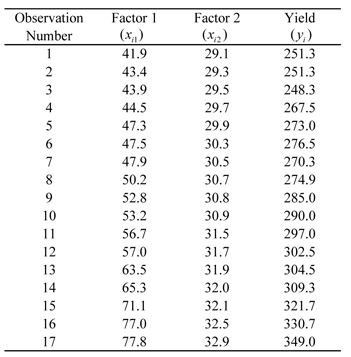
An analyst studying a chemical process expects the yield to be affected by the levels of two factors, [math]\displaystyle{ {{x}_{1}} }[/math] and [math]\displaystyle{ {{x}_{2}} }[/math] . Observations recorded for various levels of the two factors are shown in Table 5.1. The analyst wants to fit a first order regression model to the data. Interaction between [math]\displaystyle{ {{x}_{1}} }[/math] and [math]\displaystyle{ {{x}_{2}} }[/math] is not expected based on knowledge of similar processes. Units of the factor levels and the yield are ignored for the analysis.

Observed yield data for various levels of two factors.

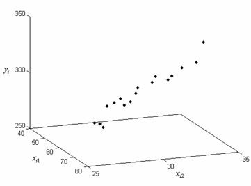
The data of Table 5.1 can be entered into DOE++ using the Multiple Regression tool as shown in Figure MLRTDataEntrySshot. A scatter plot for the data in Table 5.1 is shown in Figure ThreedScatterPlot. The first order regression model applicable to this data set having two predictor variables is:

[math]\displaystyle{ Y={{\beta }_{0}}+{{\beta }_{1}}{{x}_{1}}+{{\beta }_{2}}{{x}_{2}}+\epsilon }[/math]

where the dependent variable, [math]\displaystyle{ Y }[/math] , represents the yield and the predictor variables, [math]\displaystyle{ {{x}_{1}} }[/math] and [math]\displaystyle{ {{x}_{2}} }[/math] , represent the two factors respectively. The [math]\displaystyle{ X }[/math] and [math]\displaystyle{ y }[/math] matrices for the data can be obtained as:

[math]\displaystyle{ X=\left[ \begin{matrix} 1 & 41.9 & 29.1 \\ 1 & 43.4 & 29.3 \\ . & . & . \\ . & . & . \\ . & . & . \\ 1 & 77.8 & 32.9 \\ \end{matrix} \right]\text{ }y=\left[ \begin{matrix} 251.3 \\ 251.3 \\ . \\ . \\ . \\ 349.0 \\ \end{matrix} \right] }[/math]

Multiple Regression tool in DOE++ with the data in Table 5.1.

Three dimensional scatter plot for the observed data in Table 5.1.

The least square estimates, [math]\displaystyle{ \hat{\beta } }[/math] , can now be obtained:

[math]\displaystyle{ \begin{align} \hat{\beta } &= & {{({{X}^{\prime }}X)}^{-1}}{{X}^{\prime }}y \\ & = & {{\left[ \begin{matrix} 17 & 941 & 525.3 \\ 941 & 54270 & 29286 \\ 525.3 & 29286 & 16254 \\ \end{matrix} \right]}^{-1}}\left[ \begin{matrix} 4902.8 \\ 276610 \\ 152020 \\ \end{matrix} \right] \\ & = & \left[ \begin{matrix} -153.51 \\ 1.24 \\ 12.08 \\ \end{matrix} \right] \end{align} }[/math]

Thus:

[math]\displaystyle{ \hat{\beta }=\left[ \begin{matrix} {{{\hat{\beta }}}_{0}} \\ {{{\hat{\beta }}}_{1}} \\ {{{\hat{\beta }}}_{2}} \\ \end{matrix} \right]=\left[ \begin{matrix} -153.51 \\ 1.24 \\ 12.08 \\ \end{matrix} \right] }[/math]

and the estimated regression coefficients are [math]\displaystyle{ {{\hat{\beta }}_{0}}=-153.51 }[/math] , [math]\displaystyle{ {{\hat{\beta }}_{1}}=1.24 }[/math] and [math]\displaystyle{ {{\hat{\beta }}_{2}}=12.08 }[/math] . The fitted regression model is:

[math]\displaystyle{ \begin{align} \hat{y} & = & {{{\hat{\beta }}}_{0}}+{{{\hat{\beta }}}_{1}}{{x}_{1}}+{{{\hat{\beta }}}_{2}}{{x}_{2}} \\ & = & -153.5+1.24{{x}_{1}}+12.08{{x}_{2}} \end{align} }[/math]

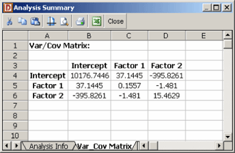
In DOE++, the fitted regression model can be viewed using the Show Analysis Summary icon in the Control Panel. The model is shown in Figure EquationScreenshot.

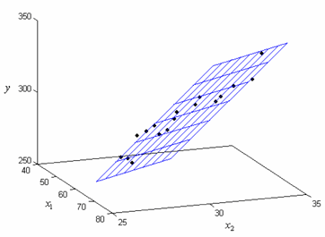
A plot of the fitted regression plane is shown in Figure FittedRegrModel. The fitted regression model can be used to obtain fitted values, [math]\displaystyle{ {{\hat{y}}_{i}} }[/math] , corresponding to an observed response value, [math]\displaystyle{ {{y}_{i}} }[/math] . For example, the fitted value corresponding to the fifth observation is:

Equation of the fitted regression model for the data in Table 5.1.

Fitted regression plane [math]\displaystyle{ \hat{y}=-153.5+1.24 x_1+12.08 x_2 }[/math] for the data of Table 5.1.

[math]\displaystyle{ \begin{align} {{{\hat{y}}}_{i}} &= & -153.5+1.24{{x}_{i1}}+12.08{{x}_{i2}} \\ {{{\hat{y}}}_{5}} & = & -153.5+1.24{{x}_{51}}+12.08{{x}_{52}} \\ & = & -153.5+1.24(47.3)+12.08(29.9) \\ & = & 266.3 \end{align} }[/math]

The observed fifth response value is [math]\displaystyle{ {{y}_{5}}=273.0 }[/math] . The residual corresponding to this value is:

[math]\displaystyle{ \begin{align} {{e}_{i}} & = & {{y}_{i}}-{{{\hat{y}}}_{i}} \\ {{e}_{5}}& = & {{y}_{5}}-{{{\hat{y}}}_{5}} \\ & = & 273.0-266.3 \\ & = & 6.7 \end{align} }[/math]

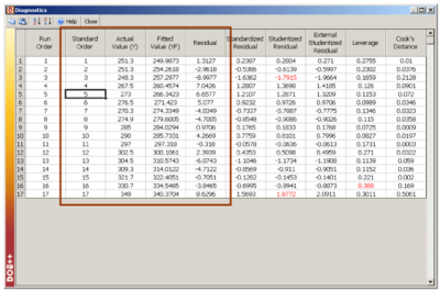
In DOE++, fitted values and residuals are available using the Diagnostic icon in the Control Panel. The values are shown in Figure DiagnosticSshot. The fitted regression model can also be used to predict response values. For example, to obtain the response value for a new observation corresponding to 47 units of [math]\displaystyle{ {{x}_{1}} }[/math] and 31 units of [math]\displaystyle{ {{x}_{2}} }[/math] , the value is calculated using:

[math]\displaystyle{ \begin{align} & \hat{y}(47,31)= & -153.5+1.24(47)+12.08(31) \\ & = & 279.26 \end{align} }[/math]

Properties of the Least Square Estimators, [math]\displaystyle{ \hat{\beta } }[/math]

The least square estimates, [math]\displaystyle{ {{\hat{\beta }}_{0}} }[/math] , [math]\displaystyle{ {{\hat{\beta }}_{1}} }[/math] , [math]\displaystyle{ {{\hat{\beta }}_{2}} }[/math] ... [math]\displaystyle{ {{\hat{\beta }}_{k}} }[/math] , are unbiased estimators of [math]\displaystyle{ {{\beta }_{0}} }[/math] , [math]\displaystyle{ {{\beta }_{1}} }[/math] , [math]\displaystyle{ {{\beta }_{2}} }[/math] ... [math]\displaystyle{ {{\beta }_{k}} }[/math] , provided that the random error terms, [math]\displaystyle{ {{\epsilon }_{i}} }[/math] , are normally and independently distributed. The variances of the [math]\displaystyle{ \hat{\beta } }[/math] s are obtained using the [math]\displaystyle{ {{({{X}^{\prime }}X)}^{-1}} }[/math] matrix. The variance-covariance matrix of the estimated regression coefficients is obtained as follows:

[math]\displaystyle{ C={{\hat{\sigma }}^{2}}{{({{X}^{\prime }}X)}^{-1}} }[/math]

Fitted values and residuals for the data in Table 5.1.

[math]\displaystyle{ C }[/math] is a symmetric matrix whose diagonal elements, [math]\displaystyle{ {{C}_{jj}} }[/math] , represent the variance of the estimated [math]\displaystyle{ j }[/math] th regression coefficient, [math]\displaystyle{ {{\hat{\beta }}_{j}} }[/math] . The off-diagonal elements, [math]\displaystyle{ {{C}_{ij}} }[/math] , represent the covariance between the [math]\displaystyle{ i }[/math] th and [math]\displaystyle{ j }[/math] th estimated regression coefficients, [math]\displaystyle{ {{\hat{\beta }}_{i}} }[/math] and [math]\displaystyle{ {{\hat{\beta }}_{j}} }[/math] . The value of [math]\displaystyle{ {{\hat{\sigma }}^{2}} }[/math] is obtained using the error mean square, [math]\displaystyle{ M{{S}_{E}} }[/math] , which can be calculated as discussed in Section 5.MANOVA. The variance-covariance matrix for the data in Table 5.1 is shown in Figure VarCovMatrixSshot. It is available in DOE++ using the Show Analysis Summary icon in the Control Panel. Calculations to obtain the matrix are given in Example 3 in Section 5.tTest. The positive square root of [math]\displaystyle{ {{C}_{jj}} }[/math] represents the estimated standard deviation of the [math]\displaystyle{ j }[/math] th regression coefficient, [math]\displaystyle{ {{\hat{\beta }}_{j}} }[/math] , and is called the estimated standard error of [math]\displaystyle{ {{\hat{\beta }}_{j}} }[/math] (abbreviated [math]\displaystyle{ se({{\hat{\beta }}_{j}}) }[/math] ).

[math]\displaystyle{ se({{\hat{\beta }}_{j}})=\sqrt{{{C}_{jj}}} }[/math]

The variance-covariance matrix for the data in Table 5.1.

Hypothesis Tests in Multiple Linear Regression

This section discusses hypothesis tests on the regression coefficients in multiple linear regression. As in the case of simple linear regression, these tests can only be carried out if it can be assumed that the random error terms, [math]\displaystyle{ {{\epsilon }_{i}} }[/math] , are normally and independently distributed with a mean of zero and variance of [math]\displaystyle{ {{\sigma }^{2}} }[/math] . Three types of hypothesis tests can be carried out for multiple linear regression models:

• Test for significance of regression

This test checks the significance of the whole regression model.

• [math]\displaystyle{ t }[/math] test

This test checks the significance of individual regression coefficients.

• Partial [math]\displaystyle{ F }[/math] test

This test can be used to simultaneously check the significance of a number of regression coefficients. It can also be used to test individual coefficients.

Test for Significance of Regression

The test for significance of regression in the case of multiple linear regression analysis is carried out using the analysis of variance. The test is used to check if a linear statistical relationship exists between the response variable and at least one of the predictor variables. The statements for the hypotheses are:

[math]\displaystyle{ \begin{align} & {{H}_{0}}: & {{\beta }_{1}}={{\beta }_{2}}=...={{\beta }_{k}}=0 \\ & {{H}_{1}}: & {{\beta }_{j}}\ne 0\text{ for at least one }j \end{align} }[/math]

The test for [math]\displaystyle{ {{H}_{0}} }[/math] is carried out using the following statistic:

[math]\displaystyle{ {{F}_{0}}=\frac{M{{S}_{R}}}{M{{S}_{E}}} }[/math]

where [math]\displaystyle{ M{{S}_{R}} }[/math] is the regression mean square and [math]\displaystyle{ M{{S}_{E}} }[/math] is the error mean square. If the null hypothesis, [math]\displaystyle{ {{H}_{0}} }[/math] , is true then the statistic [math]\displaystyle{ {{F}_{0}} }[/math] follows the [math]\displaystyle{ F }[/math] distribution with [math]\displaystyle{ k }[/math] degrees of freedom in the numerator and [math]\displaystyle{ n- }[/math] ( [math]\displaystyle{ k+1 }[/math] ) degrees of freedom in the denominator. The null hypothesis, [math]\displaystyle{ {{H}_{0}} }[/math] , is rejected if the calculated statistic, [math]\displaystyle{ {{F}_{0}} }[/math] , is such that:

[math]\displaystyle{ {{F}_{0}}\gt {{f}_{\alpha ,k,n-(k+1)}} }[/math]

Calculation of the Statistic [math]\displaystyle{ {{F}_{0}} }[/math]

To calculate the statistic [math]\displaystyle{ {{F}_{0}} }[/math] , the mean squares [math]\displaystyle{ M{{S}_{R}} }[/math] and [math]\displaystyle{ M{{S}_{E}} }[/math] must be known. As explained in Chapter 4, the mean squares are obtained by dividing the sum of squares by their degrees of freedom. For example, the total mean square, [math]\displaystyle{ M{{S}_{T}} }[/math] , is obtained as follows:

[math]\displaystyle{ M{{S}_{T}}=\frac{S{{S}_{T}}}{dof(S{{S}_{T}})} }[/math]

where [math]\displaystyle{ S{{S}_{T}} }[/math] is the total sum of squares and [math]\displaystyle{ dof(S{{S}_{T}}) }[/math] is the number of degrees of freedom associated with [math]\displaystyle{ S{{S}_{T}} }[/math] . In multiple linear regression, the following equation is used to calculate [math]\displaystyle{ S{{S}_{T}} }[/math] :

[math]\displaystyle{ S{{S}_{T}}={{y}^{\prime }}\left[ I-(\frac{1}{n})J \right]y }[/math]

where [math]\displaystyle{ n }[/math] is the total number of observations, [math]\displaystyle{ y }[/math] is the vector of observations (that was defined in Section 5.MatrixApproach), [math]\displaystyle{ I }[/math] is the identity matrix of order [math]\displaystyle{ n }[/math] and [math]\displaystyle{ J }[/math] represents an [math]\displaystyle{ n\times n }[/math] square matrix of ones. The number of degrees of freedom associated with [math]\displaystyle{ S{{S}_{T}} }[/math] , [math]\displaystyle{ dof(S{{S}_{T}}) }[/math] , is ( [math]\displaystyle{ n-1 }[/math] ). Knowing [math]\displaystyle{ S{{S}_{T}} }[/math] and [math]\displaystyle{ dof(S{{S}_{T}}) }[/math] the total mean square, [math]\displaystyle{ M{{S}_{T}} }[/math] , can be calculated.

The regression mean square, [math]\displaystyle{ M{{S}_{R}} }[/math] , is obtained by dividing the regression sum of squares, [math]\displaystyle{ S{{S}_{R}} }[/math] , by the respective degrees of freedom, [math]\displaystyle{ dof(S{{S}_{R}}) }[/math] , as follows:

[math]\displaystyle{ M{{S}_{R}}=\frac{S{{S}_{R}}}{dof(S{{S}_{R}})} }[/math]

The regression sum of squares, [math]\displaystyle{ S{{S}_{R}} }[/math] , is calculated using the following equation:

[math]\displaystyle{ S{{S}_{R}}={{y}^{\prime }}\left[ H-(\frac{1}{n})J \right]y }[/math]

where [math]\displaystyle{ n }[/math] is the total number of observations, [math]\displaystyle{ y }[/math] is the vector of observations, [math]\displaystyle{ H }[/math] is the hat matrix (that was defined in Section 5.MatrixApproach) and [math]\displaystyle{ J }[/math] represents an [math]\displaystyle{ n\times n }[/math] square matrix of ones. The number of degrees of freedom associated with [math]\displaystyle{ S{{S}_{R}} }[/math] , [math]\displaystyle{ dof(S{{S}_{E}}) }[/math] , is [math]\displaystyle{ k }[/math] , where [math]\displaystyle{ k }[/math] is the number of predictor variables in the model. Knowing [math]\displaystyle{ S{{S}_{R}} }[/math] and [math]\displaystyle{ dof(S{{S}_{R}}) }[/math] the regression mean square, [math]\displaystyle{ M{{S}_{R}} }[/math] , can be calculated. The error mean square, [math]\displaystyle{ M{{S}_{E}} }[/math] , is obtained by dividing the error sum of squares, [math]\displaystyle{ S{{S}_{E}} }[/math] , by the respective degrees of freedom, [math]\displaystyle{ dof(S{{S}_{E}}) }[/math] , as follows:

[math]\displaystyle{ M{{S}_{E}}=\frac{S{{S}_{E}}}{dof(S{{S}_{E}})} }[/math]

The error sum of squares, [math]\displaystyle{ S{{S}_{E}} }[/math] , is calculated using the following equation:

[math]\displaystyle{ S{{S}_{E}}={{y}^{\prime }}(I-H)y }[/math]

where [math]\displaystyle{ y }[/math] is the vector of observations, [math]\displaystyle{ I }[/math] is the identity matrix of order [math]\displaystyle{ n }[/math] and [math]\displaystyle{ H }[/math] is the hat matrix. The number of degrees of freedom associated with [math]\displaystyle{ S{{S}_{E}} }[/math] , [math]\displaystyle{ dof(S{{S}_{E}}) }[/math] , is [math]\displaystyle{ n-(k+1) }[/math] , where [math]\displaystyle{ n }[/math] is the total number of observations and [math]\displaystyle{ k }[/math] is the number of predictor variables in the model. Knowing [math]\displaystyle{ S{{S}_{E}} }[/math] and [math]\displaystyle{ dof(S{{S}_{E}}) }[/math] , the error mean square, [math]\displaystyle{ M{{S}_{E}} }[/math] , can be calculated. The error mean square is an estimate of the variance, [math]\displaystyle{ {{\sigma }^{2}} }[/math] , of the random error terms, [math]\displaystyle{ {{\epsilon }_{i}} }[/math] .

[math]\displaystyle{ {{\hat{\sigma }}^{2}}=M{{S}_{E}} }[/math]

Example 2

The test for the significance of regression, for the regression model obtained for the data in Table 5.1, is illustrated in this example. The null hypothesis for the model is:

[math]\displaystyle{ {{H}_{0}}\ \ :\ \ {{\beta }_{1}}={{\beta }_{2}}=0 }[/math]

The statistic to test [math]\displaystyle{ {{H}_{0}} }[/math] is:

[math]\displaystyle{ {{F}_{0}}=\frac{M{{S}_{R}}}{M{{S}_{E}}} }[/math]

To calculate [math]\displaystyle{ {{F}_{0}} }[/math] , first the sum of squares are calculated so that the mean squares can be obtained. Then the mean squares are used to calculate the statistic [math]\displaystyle{ {{F}_{0}} }[/math] to carry out the significance test. The regression sum of squares, [math]\displaystyle{ S{{S}_{R}} }[/math] , can be obtained as:

[math]\displaystyle{ S{{S}_{R}}={{y}^{\prime }}\left[ H-(\frac{1}{n})J \right]y }[/math]

The hat matrix, [math]\displaystyle{ H }[/math] is calculated as follows using the design matrix [math]\displaystyle{ X }[/math] from Example 1:

[math]\displaystyle{ \begin{align} & H= & X{{({{X}^{\prime }}X)}^{-1}}{{X}^{\prime }} \\ & = & \left[ \begin{matrix} 0.27552 & 0.25154 & . & . & -0.04030 \\ 0.25154 & 0.23021 & . & . & -0.029120 \\ . & . & . & . & . \\ . & . & . & . & . \\ -0.04030 & -0.02920 & . & . & 0.30115 \\ \end{matrix} \right] \end{align} }[/math]

Knowing [math]\displaystyle{ y }[/math] , [math]\displaystyle{ H }[/math] and [math]\displaystyle{ J }[/math] , the regression sum of squares, [math]\displaystyle{ S{{S}_{R}} }[/math] , can be calculated:

[math]\displaystyle{ \begin{align} & S{{S}_{R}}= & {{y}^{\prime }}\left[ H-(\frac{1}{n})J \right]y \\ & = & 12816.35 \end{align} }[/math]

The degrees of freedom associated with [math]\displaystyle{ S{{S}_{R}} }[/math] is [math]\displaystyle{ k }[/math] , which equals to a value of two since there are two predictor variables in the data in Table 5.1. Therefore, the regression mean square is:

[math]\displaystyle{ \begin{align} & M{{S}_{R}}= & \frac{S{{S}_{R}}}{dof(S{{S}_{R}})} \\ & = & \frac{12816.35}{2} \\ & = & 6408.17 \end{align} }[/math]

Similarly to calculate the error mean square, [math]\displaystyle{ M{{S}_{E}} }[/math] , the error sum of squares, [math]\displaystyle{ S{{S}_{E}} }[/math] , can be obtained as:

[math]\displaystyle{ \begin{align} & S{{S}_{E}}= & {{y}^{\prime }}\left[ I-H \right]y \\ & = & 423.37 \end{align} }[/math]

The degrees of freedom associated with [math]\displaystyle{ S{{S}_{E}} }[/math] is [math]\displaystyle{ n-(k+1) }[/math] . Therefore, the error mean square, [math]\displaystyle{ M{{S}_{E}} }[/math] , is:

[math]\displaystyle{ \begin{align} & M{{S}_{E}}= & \frac{S{{S}_{E}}}{dof(S{{S}_{E}})} \\ & = & \frac{S{{S}_{E}}}{(n-(k+1))} \\ & = & \frac{423.37}{(17-(2+1))} \\ & = & 30.24 \end{align} }[/math]

The statistic to test the significance of regression can now be calculated as:

[math]\displaystyle{ \begin{align} & {{f}_{0}}= & \frac{M{{S}_{R}}}{M{{S}_{E}}} \\ & = & \frac{6408.17}{423.37/(17-3)} \\ & = & 211.9 \end{align} }[/math]

The critical value for this test, corresponding to a significance level of 0.1, is:

[math]\displaystyle{ \begin{align} & {{f}_{\alpha ,k,n-(k+1)}}= & {{f}_{0.1,2,14}} \\ & = & 2.726 \end{align} }[/math]

Since [math]\displaystyle{ {{f}_{0}}\gt {{f}_{0.1,2,14}} }[/math] , [math]\displaystyle{ {{H}_{0}}\ \ : }[/math] [math]\displaystyle{ {{\beta }_{1}}={{\beta }_{2}}=0 }[/math] is rejected and it is concluded that at least one coefficient out of [math]\displaystyle{ {{\beta }_{1}} }[/math] and [math]\displaystyle{ {{\beta }_{2}} }[/math] is significant. In other words, it is concluded that a regression model exists between yield and either one or both of the factors in Table 5.1. The analysis of variance is summarized in Table 5.2.

ANOVA table for the significance of regression test in Example 2.

Test on Individual Regression Coefficients ( [math]\displaystyle{ t }[/math] Test)

The [math]\displaystyle{ t }[/math] test is used to check the significance of individual regression coefficients in the multiple linear regression model. Adding a significant variable to a regression model makes the model more effective, while adding an unimportant variable may make the model worse. The hypothesis statements to test the significance of a particular regression coefficient, [math]\displaystyle{ {{\beta }_{j}} }[/math] , are:

[math]\displaystyle{ \begin{align} & {{H}_{0}}: & {{\beta }_{j}}=0 \\ & {{H}_{1}}: & {{\beta }_{j}}\ne 0 \end{align} }[/math]

The test statistic for this test is based on the [math]\displaystyle{ t }[/math] distribution (and is similar to the one used in the case of simple linear regression models in Chapter 4):

[math]\displaystyle{ {{T}_{0}}=\frac{{{{\hat{\beta }}}_{j}}}{se({{{\hat{\beta }}}_{j}})} }[/math]

where the standard error, [math]\displaystyle{ se({{\hat{\beta }}_{j}}) }[/math] , is obtained from Eqn. (StandardErrorBetaJ). The analyst would fail to reject the null hypothesis if the test statistic, calculated using Eqn. (TtestStatistic), lies in the acceptance region:

[math]\displaystyle{ -{{t}_{\alpha /2,n-2}}\lt {{T}_{0}}\lt {{t}_{\alpha /2,n-2}} }[/math]

This test measures the contribution of a variable while the remaining variables are included in the model. For the model [math]\displaystyle{ \hat{y}={{\hat{\beta }}_{0}}+{{\hat{\beta }}_{1}}{{x}_{1}}+{{\hat{\beta }}_{2}}{{x}_{2}}+{{\hat{\beta }}_{3}}{{x}_{3}} }[/math] , if the test is carried out for [math]\displaystyle{ {{\beta }_{1}} }[/math] , then the test will check the significance of including the variable [math]\displaystyle{ {{x}_{1}} }[/math] in the model that contains [math]\displaystyle{ {{x}_{2}} }[/math] and [math]\displaystyle{ {{x}_{3}} }[/math] (i.e. the model [math]\displaystyle{ \hat{y}={{\hat{\beta }}_{0}}+{{\hat{\beta }}_{2}}{{x}_{2}}+{{\hat{\beta }}_{3}}{{x}_{3}} }[/math] ). Hence the test is also referred to as partial or marginal test. In DOE++, this test is displayed in the Regression Information table.

Example 3

The test to check the significance of the estimated regression coefficients for the data in Table 5.1 is illustrated in this example. The null hypothesis to test the coefficient [math]\displaystyle{ {{\beta }_{2}} }[/math] is:

[math]\displaystyle{ {{H}_{0}}\ \ :\ \ {{\beta }_{2}}=0 }[/math]

The null hypothesis to test [math]\displaystyle{ {{\beta }_{1}} }[/math] can be obtained in a similar manner. To calculate the test statistic, [math]\displaystyle{ {{T}_{0}} }[/math] , we need to calculate the standard error using Eqn. (StandardErrorBetaJ). In Example 2, the value of the error mean square, [math]\displaystyle{ M{{S}_{E}} }[/math] , was obtained as 30.24. The error mean square is an estimate of the variance, [math]\displaystyle{ {{\sigma }^{2}} }[/math] .

Therefore:

[math]\displaystyle{ \begin{align} & {{{\hat{\sigma }}}^{2}}= & M{{S}_{E}} \\ & = & 30.24 \end{align} }[/math]

The variance-covariance matrix of the estimated regression coefficients is:

[math]\displaystyle{ \begin{align} & C= & {{{\hat{\sigma }}}^{2}}{{({{X}^{\prime }}X)}^{-1}} \\ & = & 30.24\left[ \begin{matrix} 336.5 & 1.2 & -13.1 \\ 1.2 & 0.005 & -0.049 \\ -13.1 & -0.049 & 0.5 \\ \end{matrix} \right] \\ & = & \left[ \begin{matrix} 10176.75 & 37.145 & -395.83 \\ 37.145 & 0.1557 & -1.481 \\ -395.83 & -1.481 & 15.463 \\ \end{matrix} \right] \end{align} }[/math]

From the diagonal elements of [math]\displaystyle{ C }[/math] , the estimated standard error for [math]\displaystyle{ {{\hat{\beta }}_{1}} }[/math] and [math]\displaystyle{ {{\hat{\beta }}_{2}} }[/math] is:

[math]\displaystyle{ \begin{align} & se({{{\hat{\beta }}}_{1}})= & \sqrt{0.1557}=0.3946 \\ & se({{{\hat{\beta }}}_{2}})= & \sqrt{15.463}=3.93 \end{align} }[/math]

The corresponding test statistics for these coefficients are:

[math]\displaystyle{ \begin{align} & {{({{t}_{0}})}_{{{{\hat{\beta }}}_{1}}}}= & \frac{{{{\hat{\beta }}}_{1}}}{se({{{\hat{\beta }}}_{1}})}=\frac{1.24}{0.3946}=3.1393 \\ & {{({{t}_{0}})}_{{{{\hat{\beta }}}_{2}}}}= & \frac{{{{\hat{\beta }}}_{2}}}{se({{{\hat{\beta }}}_{2}})}=\frac{12.08}{3.93}=3.0726 \end{align} }[/math]

The critical values for the present [math]\displaystyle{ t }[/math] test at a significance of 0.1 are:

[math]\displaystyle{ \begin{align} & {{t}_{\alpha /2,n-(k+1)}}= & {{t}_{0.05,14}}=1.761 \\ & -{{t}_{\alpha /2,n-(k+1)}}= & -{{t}_{0.05,14}}=-1.761 \end{align} }[/math]

Considering [math]\displaystyle{ {{\hat{\beta }}_{2}} }[/math] , it can be seen that [math]\displaystyle{ {{({{t}_{0}})}_{{{{\hat{\beta }}}_{2}}}} }[/math] does not lie in the acceptance region of [math]\displaystyle{ -{{t}_{0.05,14}}\lt {{t}_{0}}\lt {{t}_{0.05,14}} }[/math] . The null hypothesis, [math]\displaystyle{ {{H}_{0}}\ \ :\ \ {{\beta }_{2}}=0 }[/math] , is rejected and it is concluded that [math]\displaystyle{ {{\beta }_{2}} }[/math] is significant at [math]\displaystyle{ \alpha =0.1 }[/math] . This conclusion can also be arrived at using the [math]\displaystyle{ p }[/math] value noting that the hypothesis is two-sided. The [math]\displaystyle{ p }[/math] value corresponding to the test statistic, [math]\displaystyle{ {{({{t}_{0}})}_{{{{\hat{\beta }}}_{2}}}}= }[/math] [math]\displaystyle{ 3.0726 }[/math] , based on the [math]\displaystyle{ t }[/math] distribution with 14 degrees of freedom is:

[math]\displaystyle{ \begin{align} & p\text{ }value= & 2\times (1-P(T\le |{{t}_{0}}|) \\ & = & 2\times (1-0.9959) \\ & = & 0.0083 \end{align} }[/math]

Since the [math]\displaystyle{ p }[/math] value is less than the significance, [math]\displaystyle{ \alpha =0.1 }[/math] , it is concluded that [math]\displaystyle{ {{\beta }_{2}} }[/math] is significant. The hypothesis test on [math]\displaystyle{ {{\beta }_{1}} }[/math] can be carried out in a similar manner.

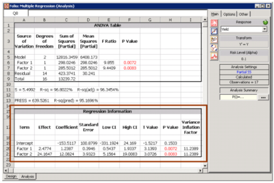
As explained in Chapter 4, in DOE++, the information related to the [math]\displaystyle{ t }[/math] test is displayed in the Regression Information table as shown in Figure RegrInfoSshot. In this table, the [math]\displaystyle{ t }[/math] test for [math]\displaystyle{ {{\beta }_{2}} }[/math] is displayed in the row for the term Factor 2 because [math]\displaystyle{ {{\beta }_{2}} }[/math] is the coefficient that represents this factor in the regression model. Columns labeled Standard Error, T Value and P Value represent the standard error, the test statistic for the [math]\displaystyle{ t }[/math] test and the [math]\displaystyle{ p }[/math] value for the [math]\displaystyle{ t }[/math] test, respectively. These values have been calculated for [math]\displaystyle{ {{\beta }_{2}} }[/math] in this example. The Coefficient column represents the estimate of regression coefficients. These values are calculated using Eqn. (LeastSquareEstimate) as shown in Example

1. The Effect column represents values obtained by multiplying the coefficients by a factor of

2. This value is useful in the case of two factor experiments and is explained in Chapter 7.

Columns labeled Low CI and High CI represent the limits of the confidence intervals for the regression coefficients and are explained in Section 5.RegrCoeffCI. The Variance Inflation Factor column displays values that give a measure of multicollinearity. This is explained in Section 5.MultiCollinearity.

Regression results for the data in Table 5.1.

Test on Subsets of Regression Coefficients (Partial [math]\displaystyle{ F }[/math] Test)

This test can be considered to be the general form of the [math]\displaystyle{ t }[/math] test mentioned in the previous section. This is because the test simultaneously checks the significance of including many (or even one) regression coefficients in the multiple linear regression model. Adding a variable to a model increases the regression sum of squares, [math]\displaystyle{ S{{S}_{R}} }[/math] . The test is based on this increase in the regression sum of squares. The increase in the regression sum of squares is called the extra sum of squares. Assume that the vector of the regression coefficients, [math]\displaystyle{ \beta }[/math] , for the multiple linear regression model, [math]\displaystyle{ y=X\beta +\epsilon }[/math] , is partitioned into two vectors with the second vector, [math]\displaystyle{ {{\beta }_{2}} }[/math] , containing the last [math]\displaystyle{ r }[/math] regression coefficients, and the first vector, [math]\displaystyle{ {{\beta }_{1}} }[/math] , containing the first ( [math]\displaystyle{ k+1-r }[/math] ) coefficients as follows:

[math]\displaystyle{ \beta =\left[ \begin{matrix} {{\beta }_{1}} \\ {{\beta }_{2}} \\ \end{matrix} \right] }[/math]

with:

[math]\displaystyle{ {{\beta }_{1}}=[{{\beta }_{0}},{{\beta }_{1}}...{{\beta }_{k-r}}{]}'\text{ and }{{\beta }_{2}}=[{{\beta }_{k-r+1}},{{\beta }_{k-r+2}}...{{\beta }_{k}}{]}'\text{ } }[/math]

The hypothesis statements to test the significance of adding the regression coefficients in [math]\displaystyle{ {{\beta }_{2}} }[/math] to a model containing the regression coefficients in [math]\displaystyle{ {{\beta }_{1}} }[/math] may be written as:

[math]\displaystyle{ \begin{align} & {{H}_{0}}: & {{\beta }_{2}}=0 \\ & {{H}_{1}}: & {{\beta }_{2}}\ne 0 \end{align} }[/math]

The test statistic for this test follows the [math]\displaystyle{ F }[/math] distribution and can be calculated as follows:

[math]\displaystyle{ {{F}_{0}}=\frac{S{{S}_{R}}({{\beta }_{2}}|{{\beta }_{1}})/r}{M{{S}_{E}}} }[/math]

where [math]\displaystyle{ S{{S}_{R}}({{\beta }_{2}}|{{\beta }_{1}}) }[/math] is the the increase in the regression sum of squares when the variables corresponding to the coefficients in [math]\displaystyle{ {{\beta }_{2}} }[/math] are added to a model already containing [math]\displaystyle{ {{\beta }_{1}} }[/math] , and [math]\displaystyle{ M{{S}_{E}} }[/math] is obtained from Eqn. (ErrorMeanSquare). The value of the extra sum of squares is obtained as explained in the next section.

The null hypothesis, [math]\displaystyle{ {{H}_{0}} }[/math] , is rejected if [math]\displaystyle{ {{F}_{0}}\gt {{f}_{\alpha ,r,n-(k+1)}} }[/math] . Rejection of [math]\displaystyle{ {{H}_{0}} }[/math] leads to the conclusion that at least one of the variables in [math]\displaystyle{ {{x}_{k-r+1}} }[/math] , [math]\displaystyle{ {{x}_{k-r+2}} }[/math] ... [math]\displaystyle{ {{x}_{k}} }[/math] contributes significantly to the regression model. In DOE++, the results from the partial [math]\displaystyle{ F }[/math] test are displayed in the ANOVA table.

Types of Extra Sum of Squares

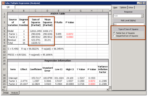
The extra sum of squares can be calculated using either the partial (or adjusted) sum of squares or the sequential sum of squares. The type of extra sum of squares used affects the calculation of the test statistic of Eqn. (PartialFtest). In DOE++, selection for the type of extra sum of squares is available in the Options tab of the Control Panel as shown in Figure SSselectionSshot. The partial sum of squares is used as the default setting. The reason for this is explained in the following section on the partial sum of squares.

Selection of the type of extra sum of squared in DOE++.

Partial Sum of Squares

The partial sum of squares for a term is the extra sum of squares when all terms, except the term under consideration, are included in the model. For example, consider the model:

[math]\displaystyle{ Y={{\beta }_{0}}+{{\beta }_{1}}{{x}_{1}}+{{\beta }_{2}}{{x}_{2}}+{{\beta }_{12}}{{x}_{1}}{{x}_{2}}+\epsilon }[/math]

Assume that we need to know the partial sum of squares for [math]\displaystyle{ {{\beta }_{2}} }[/math] . The partial sum of squares for [math]\displaystyle{ {{\beta }_{2}} }[/math] is the increase in the regression sum of squares when [math]\displaystyle{ {{\beta }_{2}} }[/math] is added to the model. This increase is the difference in the regression sum of squares for the full model of Eqn. (PartialSSFullModel) and the model that includes all terms except [math]\displaystyle{ {{\beta }_{2}} }[/math] . These terms are [math]\displaystyle{ {{\beta }_{0}} }[/math] , [math]\displaystyle{ {{\beta }_{1}} }[/math] and [math]\displaystyle{ {{\beta }_{12}} }[/math] . The model that contains these terms is:

[math]\displaystyle{ Y={{\beta }_{0}}+{{\beta }_{1}}{{x}_{1}}+{{\beta }_{12}}{{x}_{1}}{{x}_{2}}+\epsilon }[/math]

The partial sum of squares for [math]\displaystyle{ {{\beta }_{2}} }[/math] can be represented as [math]\displaystyle{ S{{S}_{R}}({{\beta }_{2}}|{{\beta }_{0}},{{\beta }_{1}},{{\beta }_{12}}) }[/math] and is calculated as follows:

[math]\displaystyle{ \begin{align} & S{{S}_{R}}({{\beta }_{2}}|{{\beta }_{0}},{{\beta }_{1}},{{\beta }_{12}})= & S{{S}_{R}}\text{ for Eqn}\text{. () }-S{{S}_{R}}\text{ for Eqn}\text{. ()} \\ & = & S{{S}_{R}}({{\beta }_{0}},{{\beta }_{1}},{{\beta }_{2}},{{\beta }_{12}})-S{{S}_{R}}({{\beta }_{0}},{{\beta }_{1}},{{\beta }_{12}}) \end{align} }[/math]

For the present case, [math]\displaystyle{ {{\beta }_{2}}=[{{\beta }_{2}}{]}' }[/math] and [math]\displaystyle{ {{\beta }_{1}}=[{{\beta }_{0}},{{\beta }_{1}},{{\beta }_{12}}{]}' }[/math] . It can be noted that for the partial sum of squares [math]\displaystyle{ {{\beta }_{1}} }[/math] contains all coefficients other than the coefficient being tested.

DOE++ has the partial sum of squares as the default selection. This is because the [math]\displaystyle{ t }[/math] test explained in Section 5.tTest is a partial test, i.e. the [math]\displaystyle{ t }[/math] test on an individual coefficient is carried by assuming that all the remaining coefficients are included in the model (similar to the way the partial sum of squares is calculated). The results from the [math]\displaystyle{ t }[/math] test are displayed in the Regression Information table. The results from the partial [math]\displaystyle{ F }[/math] test are displayed in the ANOVA table. To keep the results in the two tables consistent with each other, the partial sum of squares is used as the default selection for the results displayed in the ANOVA table. The partial sum of squares for all terms of a model may not add up to the regression sum of squares for the full model when the regression coefficients are correlated. If it is preferred that the extra sum of squares for all terms in the model always add up to the regression sum of squares for the full model then the sequential sum of squares should be used.

Example 4

This example illustrates the partial [math]\displaystyle{ F }[/math] test using the partial sum of squares. The test is conducted for the coefficient [math]\displaystyle{ {{\beta }_{1}} }[/math] corresponding to the predictor variable [math]\displaystyle{ {{x}_{1}} }[/math] for the data in Table 5.1. The regression model used for this data set in Example 1 is:

[math]\displaystyle{ Y={{\beta }_{0}}+{{\beta }_{1}}{{x}_{1}}+{{\beta }_{2}}{{x}_{2}}+\epsilon }[/math]

The null hypothesis to test the significance of [math]\displaystyle{ {{\beta }_{1}} }[/math] is:

[math]\displaystyle{ {{H}_{0}}\ \ :\ \ {{\beta }_{1}}=0 }[/math]

The statistic to test this hypothesis is:

[math]\displaystyle{ {{F}_{0}}=\frac{S{{S}_{R}}({{\beta }_{2}}|{{\beta }_{1}})/r}{M{{S}_{E}}} }[/math]

where [math]\displaystyle{ S{{S}_{R}}({{\beta }_{2}}|{{\beta }_{1}}) }[/math] represents the partial sum of squares for [math]\displaystyle{ {{\beta }_{1}} }[/math] , [math]\displaystyle{ r }[/math] represents the number of degrees of freedom for [math]\displaystyle{ S{{S}_{R}}({{\beta }_{2}}|{{\beta }_{1}}) }[/math] (which is one because there is just one coefficient, [math]\displaystyle{ {{\beta }_{1}} }[/math] , being tested) and [math]\displaystyle{ M{{S}_{E}} }[/math] is the error mean square that can obtained using Eqn. (ErrorMeanSquare) and has been calculated in Example 2 as 30.24.

The partial sum of squares for [math]\displaystyle{ {{\beta }_{1}} }[/math] is the difference between the regression sum of squares for the full model, [math]\displaystyle{ Y={{\beta }_{0}}+{{\beta }_{1}}{{x}_{1}}+{{\beta }_{2}}{{x}_{2}}+\epsilon }[/math] , and the regression sum of squares for the model excluding [math]\displaystyle{ {{\beta }_{1}} }[/math] , [math]\displaystyle{ Y={{\beta }_{0}}+{{\beta }_{2}}{{x}_{2}}+\epsilon }[/math] . The regression sum of squares for the full model can be obtained using Eqn. (TotalSumofSquares) and has been calculated in Example 2 as [math]\displaystyle{ 12816.35 }[/math] . Therefore:

[math]\displaystyle{ S{{S}_{R}}({{\beta }_{0}},{{\beta }_{1}},{{\beta }_{2}})=12816.35 }[/math]

The regression sum of squares for the model [math]\displaystyle{ Y={{\beta }_{0}}+{{\beta }_{2}}{{x}_{2}}+\epsilon }[/math] is obtained as shown next. First the design matrix for this model, [math]\displaystyle{ {{X}_{{{\beta }_{0}},{{\beta }_{2}}}} }[/math] , is obtained by dropping the second column in the design matrix of the full model, [math]\displaystyle{ X }[/math] (the full design matrix, [math]\displaystyle{ X }[/math] , was obtained in Example 1). The second column of [math]\displaystyle{ X }[/math] corresponds to the coefficient [math]\displaystyle{ {{\beta }_{1}} }[/math] which is no longer in the model. Therefore, the design matrix for the model, [math]\displaystyle{ Y={{\beta }_{0}}+{{\beta }_{2}}{{x}_{2}}+\epsilon }[/math] , is:

[math]\displaystyle{ {{X}_{{{\beta }_{0}},{{\beta }_{2}}}}=\left[ \begin{matrix} 1 & 29.1 \\ 1 & 29.3 \\ . & . \\ . & . \\ 1 & 32.9 \\ \end{matrix} \right] }[/math]

The hat matrix corresponding to this design matrix is [math]\displaystyle{ {{H}_{{{\beta }_{0}},{{\beta }_{2}}}} }[/math] . It can be calculated using [math]\displaystyle{ {{H}_{{{\beta }_{0}},{{\beta }_{2}}}}={{X}_{{{\beta }_{0}},{{\beta }_{2}}}}{{(X_{{{\beta }_{0}},{{\beta }_{2}}}^{\prime }{{X}_{{{\beta }_{0}},{{\beta }_{2}}}})}^{-1}}X_{{{\beta }_{0}},{{\beta }_{2}}}^{\prime } }[/math] . Once [math]\displaystyle{ {{H}_{{{\beta }_{0}},{{\beta }_{2}}}} }[/math] is known, the regression sum of squares for the model [math]\displaystyle{ Y={{\beta }_{0}}+{{\beta }_{2}}{{x}_{2}}+\epsilon }[/math] , can be calculated using Eqn. (RegressionSumofSquares) as:

[math]\displaystyle{ \begin{align} & S{{S}_{R}}({{\beta }_{0}},{{\beta }_{2}})= & {{y}^{\prime }}\left[ {{H}_{{{\beta }_{0}},{{\beta }_{2}}}}-(\frac{1}{n})J \right]y \\ & = & 12518.32 \end{align} }[/math]

Therefore, the partial sum of squares for [math]\displaystyle{ {{\beta }_{1}} }[/math] is:

[math]\displaystyle{ \begin{align} & S{{S}_{R}}({{\beta }_{2}}|{{\beta }_{1}})= & S{{S}_{R}}({{\beta }_{0}},{{\beta }_{1}},{{\beta }_{2}})-S{{S}_{R}}({{\beta }_{0}},{{\beta }_{2}}) \\ & = & 12816.35-12518.32 \\ & = & 298.03 \end{align} }[/math]

Knowing the partial sum of squares, the statistic to test the significance of [math]\displaystyle{ {{\beta }_{1}} }[/math] is:

[math]\displaystyle{ \begin{align} & {{f}_{0}}= & \frac{S{{S}_{R}}({{\beta }_{2}}|{{\beta }_{1}})/r}{M{{S}_{E}}} \\ & = & \frac{298.03/1}{30.24} \\ & = & 9.855 \end{align} }[/math]

The [math]\displaystyle{ p }[/math] value corresponding to this statistic based on the [math]\displaystyle{ F }[/math] distribution with 1 degree of freedom in the numerator and 14 degrees of freedom in the denominator is:

[math]\displaystyle{ \begin{align} & p\text{ }value= & 1-P(F\le {{f}_{0}}) \\ & = & 1-0.9928 \\ & = & 0.0072 \end{align} }[/math]

Assuming that the desired significance is 0.1, since [math]\displaystyle{ p }[/math] value < 0.1, [math]\displaystyle{ {{H}_{0}}\ \ :\ \ {{\beta }_{1}}=0 }[/math] is rejected and it can be concluded that [math]\displaystyle{ {{\beta }_{1}} }[/math] is significant. The test for [math]\displaystyle{ {{\beta }_{2}} }[/math] can be carried out in a similar manner. In the results obtained from DOE++, the calculations for this test are displayed in the ANOVA table as shown in Figure AnovaTableSshot. Note that the conclusion obtained in this example can also be obtained using the [math]\displaystyle{ t }[/math] test as explained in Example 3 in Section 5.tTest. The ANOVA and Regression Information tables in DOE++ represent two different ways to test for the significance of the variables included in the multiple linear regression model.

Sequential Sum of Squares

The sequential sum of squares for a coefficient is the extra sum of squares when coefficients are added to the model in a sequence. For example, consider the model:

[math]\displaystyle{ Y={{\beta }_{0}}+{{\beta }_{1}}{{x}_{1}}+{{\beta }_{2}}{{x}_{2}}+{{\beta }_{12}}{{x}_{1}}{{x}_{2}}+{{\beta }_{3}}{{x}_{3}}+{{\beta }_{13}}{{x}_{1}}{{x}_{3}}+{{\beta }_{23}}{{x}_{2}}{{x}_{3}}+{{\beta }_{123}}{{x}_{1}}{{x}_{2}}{{x}_{3}}+\epsilon }[/math]

The sequential sum of squares for [math]\displaystyle{ {{\beta }_{13}} }[/math] is the increase in the sum of squares when [math]\displaystyle{ {{\beta }_{13}} }[/math] is added to the model observing the sequence of Eqn. (SeqSSEqn). Therefore this extra sum of squares can be obtained by taking the difference between the regression sum of squares for the model after [math]\displaystyle{ {{\beta }_{13}} }[/math] was added and the regression sum of squares for the model before [math]\displaystyle{ {{\beta }_{13}} }[/math] was added to the model. The model after [math]\displaystyle{ {{\beta }_{13}} }[/math] is added is as follows:

[math]\displaystyle{ Y={{\beta }_{0}}+{{\beta }_{1}}{{x}_{1}}+{{\beta }_{2}}{{x}_{2}}+{{\beta }_{12}}{{x}_{1}}{{x}_{2}}+{{\beta }_{3}}{{x}_{3}}+{{\beta }_{13}}{{x}_{1}}{{x}_{3}}+\epsilon }[/math]

ANOVA results for the data in Table 5.1.

This is because to maintain the sequence of Eqn. (SeqSSEqn) all coefficients preceding [math]\displaystyle{ {{\beta }_{13}} }[/math] must be included in the model. These are the coefficients [math]\displaystyle{ {{\beta }_{0}} }[/math] , [math]\displaystyle{ {{\beta }_{1}} }[/math] , [math]\displaystyle{ {{\beta }_{2}} }[/math] , [math]\displaystyle{ {{\beta }_{12}} }[/math] and [math]\displaystyle{ {{\beta }_{3}} }[/math] . Similarly the model before [math]\displaystyle{ {{\beta }_{13}} }[/math] is added must contain all coefficients of Eqn. (SeqSSEqnafter) except [math]\displaystyle{ {{\beta }_{13}} }[/math] . This model can be obtained as follows:

[math]\displaystyle{ Y={{\beta }_{0}}+{{\beta }_{1}}{{x}_{1}}+{{\beta }_{2}}{{x}_{2}}+{{\beta }_{12}}{{x}_{1}}{{x}_{2}}+{{\beta }_{3}}{{x}_{3}}+\epsilon }[/math]

The sequential sum of squares for [math]\displaystyle{ {{\beta }_{13}} }[/math] can be calculated as follows:

[math]\displaystyle{ \begin{align} & S{{S}_{R}}({{\beta }_{13}}|{{\beta }_{0}},{{\beta }_{1}},{{\beta }_{2}},{{\beta }_{12}},{{\beta }_{3}})= & S{{S}_{R}}\text{ for Eqn}\text{.()}-S{{S}_{R}}\text{ for Eqn}\text{.()} \\ & = & S{{S}_{R}}({{\beta }_{0}},{{\beta }_{1}},{{\beta }_{2}},{{\beta }_{12}},{{\beta }_{3}},{{\beta }_{13}})- \\ & & S{{S}_{R}}({{\beta }_{0}},{{\beta }_{1}},{{\beta }_{2}},{{\beta }_{12}},{{\beta }_{3}}) \end{align} }[/math]

For the present case, [math]\displaystyle{ {{\beta }_{2}}=[{{\beta }_{13}}{]}' }[/math] and [math]\displaystyle{ {{\beta }_{1}}=[{{\beta }_{0}},{{\beta }_{1}},{{\beta }_{2}},{{\beta }_{12}},{{\beta }_{3}}{]}' }[/math] . It can be noted that for the sequential sum of squares [math]\displaystyle{ {{\beta }_{1}} }[/math] contains all coefficients proceeding the coefficient being tested.

The sequential sum of squares for all terms will add up to the regression sum of squares for the full model, but the sequential sum of squares are order dependent.

Example 5

This example illustrates the partial [math]\displaystyle{ F }[/math] test using the sequential sum of squares. The test is conducted for the coefficient [math]\displaystyle{ {{\beta }_{1}} }[/math] corresponding to the predictor variable [math]\displaystyle{ {{x}_{1}} }[/math] for the data in Table 5.1. The regression model used for this data set in Example 1 is:

[math]\displaystyle{ Y={{\beta }_{0}}+{{\beta }_{1}}{{x}_{1}}+{{\beta }_{2}}{{x}_{2}}+\epsilon }[/math]

The null hypothesis to test the significance of [math]\displaystyle{ {{\beta }_{1}} }[/math] is:

[math]\displaystyle{ {{H}_{0}}\ \ :\ \ {{\beta }_{1}}=0 }[/math]

The statistic to test this hypothesis is:

[math]\displaystyle{ {{F}_{0}}=\frac{S{{S}_{R}}({{\beta }_{2}}|{{\beta }_{1}})/r}{M{{S}_{E}}} }[/math]

where [math]\displaystyle{ S{{S}_{R}}({{\beta }_{2}}|{{\beta }_{1}}) }[/math] represents the sequential sum of squares for [math]\displaystyle{ {{\beta }_{1}} }[/math] , [math]\displaystyle{ r }[/math] represents the number of degrees of freedom for [math]\displaystyle{ S{{S}_{R}}({{\beta }_{2}}|{{\beta }_{1}}) }[/math] (which is one because there is just one coefficient, [math]\displaystyle{ {{\beta }_{1}} }[/math] , being tested) and [math]\displaystyle{ M{{S}_{E}} }[/math] is the error mean square that can obtained using Eqn. (ErrorMeanSquare) and has been calculated in Example 2 as 30.24.

The sequential sum of squares for [math]\displaystyle{ {{\beta }_{1}} }[/math] is the difference between the regression sum of squares for the model after adding [math]\displaystyle{ {{\beta }_{1}} }[/math] , [math]\displaystyle{ Y={{\beta }_{0}}+{{\beta }_{1}}{{x}_{1}}+\epsilon }[/math] , and the regression sum of squares for the model before adding [math]\displaystyle{ {{\beta }_{1}} }[/math] , [math]\displaystyle{ Y={{\beta }_{0}}+\epsilon }[/math] . The regression sum of squares for the model [math]\displaystyle{ Y={{\beta }_{0}}+{{\beta }_{1}}{{x}_{1}}+\epsilon }[/math] is obtained as shown next. First the design matrix for this model, [math]\displaystyle{ {{X}_{{{\beta }_{0}},{{\beta }_{1}}}} }[/math] , is obtained by dropping the third column in the design matrix for the full model, [math]\displaystyle{ X }[/math] (the full design matrix, [math]\displaystyle{ X }[/math] , was obtained in Example 1). The third column of [math]\displaystyle{ X }[/math] corresponds to coefficient [math]\displaystyle{ {{\beta }_{2}} }[/math] which is no longer used in the present model. Therefore, the design matrix for the model, [math]\displaystyle{ Y={{\beta }_{0}}+{{\beta }_{1}}{{x}_{1}}+\epsilon }[/math] , is:

[math]\displaystyle{ {{X}_{{{\beta }_{0}},{{\beta }_{1}}}}=\left[ \begin{matrix} 1 & 41.9 \\ 1 & 43.4 \\ . & . \\ . & . \\ 1 & 77.8 \\ \end{matrix} \right] }[/math]

The hat matrix corresponding to this design matrix is [math]\displaystyle{ {{H}_{{{\beta }_{0}},{{\beta }_{1}}}} }[/math] . It can be calculated using [math]\displaystyle{ {{H}_{{{\beta }_{0}},{{\beta }_{1}}}}={{X}_{{{\beta }_{0}},{{\beta }_{1}}}}{{(X_{{{\beta }_{0}},{{\beta }_{1}}}^{\prime }{{X}_{{{\beta }_{0}},{{\beta }_{1}}}})}^{-1}}X_{{{\beta }_{0}},{{\beta }_{1}}}^{\prime } }[/math] . Once [math]\displaystyle{ {{H}_{{{\beta }_{0}},{{\beta }_{1}}}} }[/math] is known, the regression sum of squares for the model [math]\displaystyle{ Y={{\beta }_{0}}+{{\beta }_{1}}{{x}_{1}}+\epsilon }[/math] can be calculated using Eqn. (RegressionSumofSquares) as:

[math]\displaystyle{ \begin{align} & S{{S}_{R}}({{\beta }_{0}},{{\beta }_{1}})= & {{y}^{\prime }}\left[ {{H}_{{{\beta }_{0}},{{\beta }_{1}}}}-(\frac{1}{n})J \right]y \\ & = & 12530.85 \end{align} }[/math]

Sequential sum of squares for the data in Table 5.1.

The regression sum of squares for the model [math]\displaystyle{ Y={{\beta }_{0}}+\epsilon }[/math] is equal to zero since this model does not contain any variables. Therefore:

[math]\displaystyle{ S{{S}_{R}}({{\beta }_{0}})=0 }[/math]

The sequential sum of squares for [math]\displaystyle{ {{\beta }_{1}} }[/math] is:

[math]\displaystyle{ \begin{align} & S{{S}_{R}}({{\beta }_{2}}|{{\beta }_{1}})= & S{{S}_{R}}({{\beta }_{0}},{{\beta }_{1}})-S{{S}_{R}}({{\beta }_{0}}) \\ & = & 12530.85-0 \\ & = & 12530.85 \end{align} }[/math]

Knowing the sequential sum of squares, the statistic to test the significance of [math]\displaystyle{ {{\beta }_{1}} }[/math] is:

[math]\displaystyle{ \begin{align} & {{f}_{0}}= & \frac{S{{S}_{R}}({{\beta }_{2}}|{{\beta }_{1}})/r}{M{{S}_{E}}} \\ & = & \frac{12530.85/1}{30.24} \\ & = & 414.366 \end{align} }[/math]

The [math]\displaystyle{ p }[/math] value corresponding to this statistic based on the [math]\displaystyle{ F }[/math] distribution with 1 degree of freedom in the numerator and 14 degrees of freedom in the denominator is:

[math]\displaystyle{ \begin{align} & p\text{ }value= & 1-P(F\le {{f}_{0}}) \\ & = & 1-0.999999 \\ & = & 8.46\times {{10}^{-12}} \end{align} }[/math]

Assuming that the desired significance is 0.1, since [math]\displaystyle{ p }[/math] value < 0.1, [math]\displaystyle{ {{H}_{0}}\ \ :\ \ {{\beta }_{1}}=0 }[/math] is rejected and it can be concluded that [math]\displaystyle{ {{\beta }_{1}} }[/math] is significant. The test for [math]\displaystyle{ {{\beta }_{2}} }[/math] can be carried out in a similar manner. This result is shown in Figure SequentialSshot.

Confidence Intervals in Multiple Linear Regression

Calculation of confidence intervals for multiple linear regression models are similar to those for simple linear regression models explained in Chapter 4.

Confidence Interval on Regression Coefficients

A 100( [math]\displaystyle{ 1-\alpha }[/math] ) percent confidence interval on the regression coefficient, [math]\displaystyle{ {{\beta }_{j}} }[/math] , is obtained as follows:

[math]\displaystyle{ {{\hat{\beta }}_{j}}\pm {{t}_{\alpha /2,n-(k+1)}}\sqrt{{{C}_{jj}}} }[/math]

The confidence interval on the regression coefficients are displayed in the Regression Information table under the Low CI and High CI columns as shown in Figure RegrInfoSshot. Confidence Interval on Fitted Values, [math]\displaystyle{ {{\hat{y}}_{i}} }[/math] A 100( [math]\displaystyle{ 1-\alpha }[/math] ) percent confidence interval on any fitted value, [math]\displaystyle{ {{\hat{y}}_{i}} }[/math] , is given by:

[math]\displaystyle{ {{\hat{y}}_{i}}\pm {{t}_{\alpha /2,n-(k+1)}}\sqrt{{{{\hat{\sigma }}}^{2}}x_{i}^{\prime }{{({{X}^{\prime }}X)}^{-1}}{{x}_{i}}} }[/math]

where:

[math]\displaystyle{ {{x}_{i}}=\left[ \begin{matrix} 1 \\ {{x}_{i1}} \\ . \\ . \\ . \\ {{x}_{ik}} \\ \end{matrix} \right] }[/math]

In Example 1 (Section 5.MatrixApproach), the fitted value corresponding to the fifth observation was calculated as [math]\displaystyle{ {{\hat{y}}_{5}}=266.3 }[/math] . The 90% confidence interval on this value can be obtained as shown in Figure CIfittedvalueSshot. The values of 47.3 and 29.9 used in the figure are the values of the predictor variables corresponding to the fifth observation in Table 5.1.

Confidence interval for the fitted value corresponding to the fifth observation in Table 5.1.

Confidence Interval on New Observations

As explained in Chapter 4, the confidence interval on a new observation is also referred to as the prediction interval. The prediction interval takes into account both the error from the fitted model and the error associated with future observations. A 100( [math]\displaystyle{ 1-\alpha }[/math] ) percent confidence interval on a new observation, [math]\displaystyle{ {{\hat{y}}_{p}} }[/math] , is obtained as follows:

[math]\displaystyle{ {{\hat{y}}_{p}}\pm {{t}_{\alpha /2,n-(k+1)}}\sqrt{{{{\hat{\sigma }}}^{2}}(1+x_{p}^{\prime }{{({{X}^{\prime }}X)}^{-1}}{{x}_{p}})} }[/math]

where:

[math]\displaystyle{ {{x}_{p}}=\left[ \begin{matrix} 1 \\ {{x}_{p1}} \\ . \\ . \\ . \\ {{x}_{pk}} \\ \end{matrix} \right] }[/math]

[math]\displaystyle{ {{x}_{p1}} }[/math] ,..., [math]\displaystyle{ {{x}_{pk}} }[/math] are the levels of the predictor variables at which the new observation, [math]\displaystyle{ {{\hat{y}}_{p}} }[/math] , needs to be obtained.

Predicted values and region of model application in multiple linear regression.

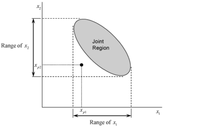
In multiple linear regression, prediction intervals should only be obtained at the levels of the predictor variables where the regression model applies. In the case of multiple linear regression it is easy to miss this. Having values lying within the range of the predictor variables does not necessarily mean that the new observation lies in the region to which the model is applicable. For example, consider Figure JointRegion where the shaded area shows the region to which a two variable regression model is applicable. The point corresponding to [math]\displaystyle{ p }[/math] th level of first predictor variable, [math]\displaystyle{ {{x}_{1}} }[/math] , and [math]\displaystyle{ p }[/math] th level of the second predictor variable, [math]\displaystyle{ {{x}_{2}} }[/math] , does not lie in the shaded area, although both of these levels are within the range of the first and second predictor variables respectively. In this case, the regression model is not applicable at this point.

Measures of Model Adequacy

As in the case of simple linear regression, analysis of a fitted multiple linear regression model is important before inferences based on the model are undertaken. This section presents some techniques that can be used to check the appropriateness of the multiple linear regression model.

Coefficient of Multiple Determination, [math]\displaystyle{ {{R}^{2}} }[/math]

The coefficient of multiple determination is similar to the coefficient of determination used in the case of simple linear regression. It is defined as:

[math]\displaystyle{ \begin{align} & {{R}^{2}}= & \frac{S{{S}_{R}}}{S{{S}_{T}}} \\ & = & 1-\frac{S{{S}_{E}}}{S{{S}_{T}}} \end{align} }[/math]

[math]\displaystyle{ {{R}^{2}} }[/math] indicates the amount of total variability explained by the regression model. The positive square root of [math]\displaystyle{ {{R}^{2}} }[/math] is called the multiple correlation coefficient and measures the linear association between [math]\displaystyle{ Y }[/math] and the predictor variables, [math]\displaystyle{ {{x}_{1}} }[/math] , [math]\displaystyle{ {{x}_{2}} }[/math] ... [math]\displaystyle{ {{x}_{k}} }[/math] .

The value of [math]\displaystyle{ {{R}^{2}} }[/math] increases as more terms are added to the model, even if the new term does not contribute significantly to the model. An increase in the value of [math]\displaystyle{ {{R}^{2}} }[/math] cannot be taken as a sign to conclude that the new model is superior to the older model. A better statistic to use is the adjusted [math]\displaystyle{ {{R}^{2}} }[/math] statistic defined as follows:

[math]\displaystyle{ \begin{align} & R_{adj}^{2}= & 1-\frac{M{{S}_{E}}}{M{{S}_{T}}} \\ & = & 1-\frac{S{{S}_{E}}/(n-(k+1))}{S{{S}_{T}}/(n-1)} \\ & = & 1-(\frac{n-1}{n-(k+1)})(1-{{R}^{2}}) \end{align} }[/math]

The adjusted [math]\displaystyle{ {{R}^{2}} }[/math] only increases when significant terms are added to the model. Addition of unimportant terms may lead to a decrease in the value of [math]\displaystyle{ R_{adj}^{2} }[/math] .

In DOE++, [math]\displaystyle{ {{R}^{2}} }[/math] and [math]\displaystyle{ R_{adj}^{2} }[/math] values are displayed as R-sq and R-sq(adj), respectively. Other values displayed along with these values are S, PRESS and R-sq(pred). As explained in Chapter 4, the value of S is the square root of the error mean square, [math]\displaystyle{ M{{S}_{E}} }[/math] , and represents the "standard error of the model."

PRESS is an abbreviation for prediction error sum of squares. It is the error sum of squares calculated using the PRESS residuals in place of the residuals, [math]\displaystyle{ {{e}_{i}} }[/math] , in Eqn. (ErrorSumofSquares). The PRESS residual, [math]\displaystyle{ {{e}_{(i)}} }[/math] , for a particular observation, [math]\displaystyle{ {{y}_{i}} }[/math] , is obtained by fitting the regression model to the remaining observations. Then the value for a new observation, [math]\displaystyle{ {{\hat{y}}_{p}} }[/math] , corresponding to the observation in question, [math]\displaystyle{ {{y}_{i}} }[/math] , is obtained based on the new regression model. The difference between [math]\displaystyle{ {{y}_{i}} }[/math] and [math]\displaystyle{ {{\hat{y}}_{p}} }[/math] gives [math]\displaystyle{ {{e}_{(i)}} }[/math] . The PRESS residual, [math]\displaystyle{ {{e}_{(i)}} }[/math] , can also be obtained using [math]\displaystyle{ {{h}_{ii}} }[/math] , the diagonal element of the hat matrix, [math]\displaystyle{ H }[/math] , as follows:

[math]\displaystyle{ {{e}_{(i)}}=\frac{{{e}_{i}}}{1-{{h}_{ii}}} }[/math]

R-sq(pred), also referred to as prediction [math]\displaystyle{ {{R}^{2}} }[/math] , is obtained using PRESS as shown next:

[math]\displaystyle{ R_{pred}^{2}=1-\frac{PRESS}{S{{S}_{T}}} }[/math]

The values of R-sq, R-sq(adj) and S are indicators of how well the regression model fits the observed data. The values of PRESS and R-sq(pred) are indicators of how well the regression model predicts new observations. For example, higher values of PRESS or lower values of R-sq(pred) indicate a model that predicts poorly. Figure RSqadjSshot. shows these values for the data in Table 5.1. The values indicate that the regression model fits the data well and also predicts well.

Residual Analysis

Plots of residuals, [math]\displaystyle{ {{e}_{i}} }[/math] , similar to the ones discussed in the previous chapter for simple linear regression, are used to check the adequacy of a fitted multiple linear regression model. The residuals are expected to be normally distributed with a mean of zero and a constant variance of [math]\displaystyle{ {{\sigma }^{2}} }[/math] . In addition, they should not show any patterns or trends when plotted against any variable or in a time or run-order sequence. Residual plots may also be obtained using standardized and studentized residuals. Standardized residuals, [math]\displaystyle{ {{d}_{i}} }[/math] , are obtained using the following equation:

[math]\displaystyle{ \begin{align} & {{d}_{i}}= & \frac{{{e}_{i}}}{\sqrt{{{{\hat{\sigma }}}^{2}}}} \\ & = & \frac{{{e}_{i}}}{\sqrt{M{{S}_{E}}}} \end{align} }[/math]

Coefficient of multiple determination and related results for the data in Table 5.1.

Standardized residuals are scaled so that the standard deviation of the residuals is approximately equal to one. This helps to identify possible outliers or unusual observations. However, standardized residuals may understate the true residual magnitude, hence studentized residuals, [math]\displaystyle{ {{r}_{i}} }[/math] , are used in their place. Studentized residuals are calculated as follows:

[math]\displaystyle{ \begin{align} & {{r}_{i}}= & \frac{{{e}_{i}}}{\sqrt{{{{\hat{\sigma }}}^{2}}(1-{{h}_{ii}})}} \\ & = & \frac{{{e}_{i}}}{\sqrt{M{{S}_{E}}(1-{{h}_{ii}})}} \end{align} }[/math]

where [math]\displaystyle{ {{h}_{ii}} }[/math] is the [math]\displaystyle{ i }[/math] th diagonal element of the hat matrix, [math]\displaystyle{ H }[/math] . External studentized (or the studentized deleted) residuals may also be used. These residuals are based on the PRESS residuals mentioned in Section 5.Rsquare. The reason for using the external studentized residuals is that if the [math]\displaystyle{ i }[/math] th observation is an outlier, it may influence the fitted model. In this case, the residual [math]\displaystyle{ {{e}_{i}} }[/math] will be small and may not disclose that [math]\displaystyle{ i }[/math] th observation is an outlier. The external studentized residual for the [math]\displaystyle{ i }[/math] th observation, [math]\displaystyle{ {{t}_{i}} }[/math] , is obtained as follows:

[math]\displaystyle{ {{t}_{i}}={{e}_{i}}{{\left[ \frac{n-k}{S{{S}_{E}}(1-{{h}_{ii}})-e_{i}^{2}} \right]}^{0.5}} }[/math]

Residual values for the data of Table 5.1 are shown in Figure ResidualSshot. These values are available using the Diagnostics icon in the Control Panel. Standardized residual plots for the data are shown in Figures Res1NPP to ResVsRuns. DOE++ compares the residual values to the critical values on the [math]\displaystyle{ t }[/math] distribution for studentized and external studentized residuals. For other residuals the normal distribution is used. For example, for the data in Table 5.1, the critical values on the [math]\displaystyle{ t }[/math] distribution at a significance of 0.1 are [math]\displaystyle{ {{t}_{0.05,14}}=1.761 }[/math] and [math]\displaystyle{ -{{t}_{0.05,14}}=-1.761 }[/math] (as calculated in Example 3, Section 5.tTest). The studentized residual values corresponding to the 3rd and 17th observations lie outside the critical values. Therefore, the 3rd and 17th observations are outliers. This can also be seen on the residual plots in Figures ResVsFitted and ResVsRuns.

Outlying [math]\displaystyle{ x }[/math] Observations

Residuals help to identify outlying [math]\displaystyle{ y }[/math] observations. Outlying [math]\displaystyle{ x }[/math] observations can be detected using leverage. Leverage values are the diagonal elements of the hat matrix, [math]\displaystyle{ {{h}_{ii}} }[/math] . The [math]\displaystyle{ {{h}_{ii}} }[/math] values always lie between 0 and 1. Values of [math]\displaystyle{ {{h}_{ii}} }[/math] greater than [math]\displaystyle{ 2(k+1)/n }[/math] are considered to be indicators of outlying [math]\displaystyle{ x }[/math] observations.

Influential Observations Detection

Once an outlier is identified, it is important to determine if the outlier has a significant effect on the regression model. One measure to detect influential observations is Cook's distance measure which is computed as follows:

[math]\displaystyle{ {{D}_{i}}=\frac{r_{i}^{2}}{(k+1)}\left[ \frac{{{h}_{ii}}}{(1-{{h}_{ii}})} \right] }[/math]

To use Cook's distance measure, the [math]\displaystyle{ {{D}_{i}} }[/math] values are compared to percentile values on the [math]\displaystyle{ F }[/math] distribution with [math]\displaystyle{ (k+1,n-(k+1)) }[/math] degrees of freedom. If the percentile value is less than 10 or 20 percent, then the [math]\displaystyle{ i }[/math] th case has little influence on the fitted values. However, if the percentile value is close to 50 percent or greater, the [math]\displaystyle{ i }[/math] th case is influential, and fitted values with and without the [math]\displaystyle{ i }[/math] th case will differ substantially.[Kutner]

Example 6

Cook's distance measure can be calculated as shown next. The distance measure is calculated for the first observation of the data in Table 5.1. The remaining values along with the leverage values are shown in Figure CookSshot. The standardized residual corresponding to the first observation is:

Residual values for the data in Table 5.1.

Residual probability plot for the data in Table 5.1.

Residual versus fitted values plot for the data in Table 5.1.

Residual versus run order plot for the data in Table 5.1.

[math]\displaystyle{ \begin{align} & {{r}_{1}}= & \frac{{{e}_{1}}}{\sqrt{M{{S}_{E}}(1-{{h}_{11}})}} \\ & = & \frac{1.3127}{\sqrt{30.3(1-0.2755)}} \\ & = & 0.2804 \end{align} }[/math]

Cook's distance measure for the first observation can now be calculated as:

[math]\displaystyle{ \begin{align} & {{D}_{1}}= & \frac{r_{1}^{2}}{(k+1)}\left[ \frac{{{h}_{11}}}{(1-{{h}_{11}})} \right] \\ & = & \frac{{{0.2804}^{2}}}{(2+1)}\left[ \frac{0.2755}{(1-0.2755)} \right] \\ & = & 0.01 \end{align} }[/math]

The 50th percentile value for [math]\displaystyle{ {{F}_{3,14}} }[/math] is 0.83. Since all [math]\displaystyle{ {{D}_{i}} }[/math] values are less than this value there are no influential observations.

Leverage and Cook's distance measure for the data in Table 5.1.

Lack-of-Fit Test

The lack-of-fit test for simple linear regression discussed in Chapter 4 may also be applied to multiple linear regression to check the appropriateness of the fitted response surface and see if a higher order model is required. Data for [math]\displaystyle{ m }[/math] replicates may be collected as follows for all [math]\displaystyle{ n }[/math] levels of the predictor variables:

[math]\displaystyle{ \begin{align} & & {{y}_{11}},{{y}_{12}},....,{{y}_{1m}}\text{ }m\text{ repeated observations at the first level } \\ & & {{y}_{21}},{{y}_{22}},....,{{y}_{2m}}\text{ }m\text{ repeated observations at the second level} \\ & & ... \\ & & {{y}_{i1}},{{y}_{i2}},....,{{y}_{im}}\text{ }m\text{ repeated observations at the }i\text{th level} \\ & & ... \\ & & {{y}_{n1}},{{y}_{n2}},....,{{y}_{nm}}\text{ }m\text{ repeated observations at the }n\text{th level } \end{align} }[/math]

The sum of squares due to pure error, [math]\displaystyle{ S{{S}_{PE}} }[/math] , can be obtained as discussed in the previous chapter as:

[math]\displaystyle{ S{{S}_{PE}}=\underset{i=1}{\overset{n}{\mathop \sum }}\,\underset{j=1}{\overset{m}{\mathop \sum }}\,{{({{y}_{ij}}-{{\bar{y}}_{i}})}^{2}} }[/math]

The number of degrees of freedom associated with [math]\displaystyle{ S{{S}_{PE}} }[/math] are:

[math]\displaystyle{ dof(S{{S}_{PE}})=nm-n }[/math]

Knowing [math]\displaystyle{ S{{S}_{PE}} }[/math] , sum of squares due to lack-of-fit, [math]\displaystyle{ S{{S}_{LOF}} }[/math] , can be obtained as:

[math]\displaystyle{ S{{S}_{LOF}}=S{{S}_{E}}-S{{S}_{PE}} }[/math]

The number of degrees of freedom associated with [math]\displaystyle{ S{{S}_{LOF}} }[/math] are:

[math]\displaystyle{ \begin{align} & dof(S{{S}_{LOF}})= & dof(S{{S}_{E}})-dof(S{{S}_{PE}}) \\ & = & n-(k+1)-(nm-n) \end{align} }[/math]

The test statistic for the lack-of-fit test is:

[math]\displaystyle{ \begin{align} & {{F}_{0}}= & \frac{S{{S}_{LOF}}/dof(S{{S}_{LOF}})}{S{{S}_{PE}}/dof(S{{S}_{PE}})} \\ & = & \frac{M{{S}_{LOF}}}{M{{S}_{PE}}} \end{align} }[/math]

Other Topics in Multiple Linear Regression

Polynomial Regression Models

Polynomial regression models are used when the response is curvilinear. The equation shown next presents a second order polynomial regression model with one predictor variable:

[math]\displaystyle{ Y={{\beta }_{0}}+{{\beta }_{1}}{{x}_{1}}+{{\beta }_{11}}x_{1}^{2}+\epsilon }[/math]

Usually, coded values are used in these models. Values of the variables are coded by centering or expressing the levels of the variable as deviations from the mean value of the variable and then scaling or dividing the deviations obtained by half of the range of the variable.

[math]\displaystyle{ coded\text{ }value=\frac{actual\text{ }value-mean}{half\text{ }of\text{ }range} }[/math]

The reason for using coded predictor variables is that many times [math]\displaystyle{ x }[/math] and [math]\displaystyle{ {{x}^{2}} }[/math] are highly correlated and, if uncoded values are used, there may be computational difficulties while calculating the [math]\displaystyle{ {{({{X}^{\prime }}X)}^{-1}} }[/math] matrix to obtain the estimates, [math]\displaystyle{ \hat{\beta } }[/math] , of the regression coefficients using Eqn. (LeastSquareEstimate).

Qualitative Factors

The multiple linear regression model also supports the use of qualitative factors. For example, gender may need to be included as a factor in a regression model. One of the ways to include qualitative factors in a regression model is to employ indicator variables. Indicator variables take on values of 0 or 1. For example, an indicator variable may be used with a value of 1 to indicate female and a value of 0 to indicate male.

[math]\displaystyle{ {{x}_{1}}=\{\begin{array}{*{35}{l}} 1\text{ Female} \\ 0\text{ Male} \\ \end{array} }[/math]

In general ( [math]\displaystyle{ n-1 }[/math] ) indicator variables are required to represent a qualitative factor with [math]\displaystyle{ n }[/math] levels. As an example, a qualitative factor representing three types of machines may be represented as follows using two indicator variables:

[math]\displaystyle{ \begin{align} & {{x}_{1}}= & 1,\text{ }{{x}_{2}}=0\text{ Machine Type I} \\ & {{x}_{1}}= & 0,\text{ }{{x}_{2}}=1\text{ Machine Type II} \\ & {{x}_{1}}= & 0,\text{ }{{x}_{2}}=0\text{ Machine Type III} \end{align} }[/math]

An alternative coding scheme for this example is to use a value of -1 for all indicator variables when representing the last level of the factor:

[math]\displaystyle{ \begin{align} & {{x}_{1}}= & 1,\text{ }{{x}_{2}}=0\text{ Machine Type I} \\ & {{x}_{1}}= & 0,\text{ }{{x}_{2}}=1\text{ Machine Type II} \\ & {{x}_{1}}= & -1,\text{ }{{x}_{2}}=-1\text{ Machine Type III} \end{align} }[/math]

Indicator variables are also referred to as dummy variables or binary variables.

Example 7

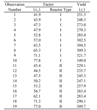
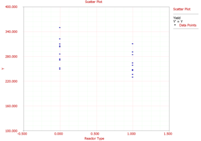
Consider data from two types of reactors of a chemical process shown in Table 5.3 where the yield values are recorded for various levels of factor [math]\displaystyle{ {{x}_{1}} }[/math] . Assuming there are no interactions between the reactor type and [math]\displaystyle{ {{x}_{1}} }[/math] , a regression model can be fitted to this data as shown next. Since the reactor type is a qualitative factor with two levels, it can be represented by using one indicator variable. Let [math]\displaystyle{ {{x}_{2}} }[/math] be the indicator variable representing the reactor type, with 0 representing the first type of reactor and 1 representing the second type of reactor.

[math]\displaystyle{ {{x}_{2}}=\{\begin{array}{*{35}{l}} 0\text{ Reactor Type I} \\ 1\text{ Reactor Type II} \\ \end{array} }[/math]

Yield data from the two types of reactors for a chemical process.

Data entry in DOE++ for this example is shown in Figure IndiVarDesignSshot. The regression model for this data is:

[math]\displaystyle{ Y={{\beta }_{0}}+{{\beta }_{1}}{{x}_{1}}+{{\beta }_{2}}{{x}_{2}}+\epsilon }[/math]

The [math]\displaystyle{ X }[/math] and [math]\displaystyle{ y }[/math] matrices for the given data are:

Data from Table 5.3 as entered in DOE++.

The estimated regression coefficients for the model can be obtained using Eqn. (LeastSquareEstimate) as:

[math]\displaystyle{ \begin{align} & \hat{\beta }= & {{({{X}^{\prime }}X)}^{-1}}{{X}^{\prime }}y \\ & = & \left[ \begin{matrix} 153.7 \\ 2.4 \\ -27.5 \\ \end{matrix} \right] \end{align} }[/math]

Therefore, the fitted regression model is:

[math]\displaystyle{ \hat{y}=153.7+2.4{{x}_{1}}-27.5{{x}_{2}} }[/math]

Note that since [math]\displaystyle{ {{x}_{2}} }[/math] represents a qualitative predictor variable, the fitted regression model cannot be plotted simultaneously against [math]\displaystyle{ {{x}_{1}} }[/math] and [math]\displaystyle{ {{x}_{2}} }[/math] in a two dimensional space (because the resulting surface plot will be meaningless for the dimension in [math]\displaystyle{ {{x}_{2}} }[/math] ). To illustrate this, a scatter plot of the data in Table 5.3 against [math]\displaystyle{ {{x}_{2}} }[/math] is shown in Figure IndiVarScatterPlot. It can be noted that, in the case of qualitative factors, the nature of the relationship between the response (yield) and the qualitative factor (reactor type) cannot be categorized as linear, or quadratic, or cubic, etc. The only conclusion that can be arrived at for these factors is to see if these factors contribute significantly to the regression model. This can be done by employing the partial [math]\displaystyle{ F }[/math] test of Section 5.FtestPartial (using the extra sum of squares of the indicator variables representing these factors). The results of the test for the present example are shown in the ANOVA table of Figure IndiVarResultsSshot. The results show that [math]\displaystyle{ {{x}_{2}} }[/math] (reactor type) contributes significantly to the fitted regression model.

Multicollinearity

At times the predictor variables included in a multiple linear regression model may be found to be dependent on each other. Multicollinearity is said to exist in a multiple regression model with strong dependencies between the predictor variables. Multicollinearity affects the regression coefficients and the extra sum of squares of the predictor variables. In a model with multicollinearity the estimate of the regression coefficient of a predictor variable depends on what other predictor variables are included the model. The dependence may even lead to change in the sign of the regression coefficient. In a such models, an estimated regression coefficient may not be found to be significant individually (when using the [math]\displaystyle{ t }[/math] test on the individual coefficient or looking at the [math]\displaystyle{ p }[/math] value) even though a statistical relation is found to exist between the response variable and the set of the predictor variables (when using the [math]\displaystyle{ F }[/math] test for the set of predictor variables). Therefore, you should be careful while looking at individual predictor variables in models that have multicollinearity. Care should also be taken while looking at the extra sum of squares for a predictor variable that is correlated with other variables. This is because in models with multicollinearity the extra sum of squares is not unique and depends on the other predictor variables included in the model.

Scatter plot of the observed yield values in Table 5.3 against [math]\displaystyle{ x_2 }[/math] (reactor type)

DOE++ results for the data in Table 5.3.

Multicollinearity can be detected using the variance inflation factor (abbreviated [math]\displaystyle{ VIF }[/math] ). [math]\displaystyle{ VIF }[/math] for a coefficient [math]\displaystyle{ {{\beta }_{j}} }[/math] is defined as:

[math]\displaystyle{ VIF=\frac{1}{(1-R_{j}^{2})} }[/math]

where [math]\displaystyle{ R_{j}^{2} }[/math] is the coefficient of multiple determination resulting from regressing the [math]\displaystyle{ j }[/math] th predictor variable, [math]\displaystyle{ {{x}_{j}} }[/math] , on the remaining [math]\displaystyle{ k }[/math] -1 predictor variables. Mean values of [math]\displaystyle{ VIF }[/math] considerably greater than 1 indicate multicollinearity problems. A few methods of dealing with multicollinearity include increasing the number of observations in a way designed to break up dependencies among predictor variables, combining the linearly dependent predictor variables into one variable, eliminating variables from the model that are unimportant or using coded variables.

Example 8

Variance inflation factors can be obtained for the data in Table 5.1. To calculate the variance inflation factor for [math]\displaystyle{ {{x}_{1}} }[/math] , [math]\displaystyle{ R_{1}^{2} }[/math] has to be calculated. [math]\displaystyle{ R_{1}^{2} }[/math] is the coefficient of determination for the model when [math]\displaystyle{ {{x}_{1}} }[/math] is regressed on the remaining variables. In the case of this example there is just one remaining variable which is [math]\displaystyle{ {{x}_{2}} }[/math] . If a regression model is fit to the data, taking [math]\displaystyle{ {{x}_{1}} }[/math] as the response variable and [math]\displaystyle{ {{x}_{2}} }[/math] as the predictor variable, then the design matrix and the vector of observations are:

[math]\displaystyle{ {{X}_{{{R}_{1}}}}=\left[ \begin{matrix} 1 & 29.1 \\ 1 & 29.3 \\ . & . \\ . & . \\ . & . \\ 1 & 32.9 \\ \end{matrix} \right]\text{ }{{y}_{{{R}_{1}}}}=\left[ \begin{matrix} 41.9 \\ 43.4 \\ . \\ . \\ . \\ 77.8 \\ \end{matrix} \right] }[/math]

The regression sum of squares for this model can be obtained using Eqn. (RegressionSumofSquares) as:

[math]\displaystyle{ \begin{align} & S{{S}_{R}}= & y_{{{R}_{1}}}^{\prime }\left[ {{H}_{{{R}_{1}}}}-(\frac{1}{n})J \right]{{y}_{{{R}_{1}}}} \\ & = & 1988.6 \end{align} }[/math]

where [math]\displaystyle{ {{H}_{{{R}_{1}}}} }[/math] is the hat matrix (and is calculated using [math]\displaystyle{ {{H}_{{{R}_{1}}}}={{X}_{{{R}_{1}}}}{{(X_{{{R}_{1}}}^{\prime }{{X}_{{{R}_{1}}}})}^{-1}}X_{{{R}_{1}}}^{\prime } }[/math] ) and [math]\displaystyle{ J }[/math] is the matrix of ones. The total sum of squares for the model can be calculated using Eqn. (TotalSumofSquares) as:

[math]\displaystyle{ \begin{align} & S{{S}_{T}}= & {{y}^{\prime }}\left[ I-(\frac{1}{n})J \right]y \\ & = & 2182.9 \end{align} }[/math]

where [math]\displaystyle{ I }[/math] is the identity matrix. Therefore:

[math]\displaystyle{ \begin{align} & R_{1}^{2}= & \frac{S{{S}_{R}}}{S{{S}_{T}}} \\ & = & \frac{1988.6}{2182.9} \\ & = & 0.911 \end{align} }[/math]

Then the variance inflation factor for [math]\displaystyle{ {{x}_{1}} }[/math] is:

[math]\displaystyle{ \begin{align} & VI{{F}_{1}}= & \frac{1}{(1-R_{1}^{2})} \\ & = & \frac{1}{1-0.911} \\ & = & 11.2 \end{align} }[/math]

The variance inflation factor for [math]\displaystyle{ {{x}_{2}} }[/math] , [math]\displaystyle{ VI{{F}_{2}} }[/math] , can be obtained in a similar manner. In DOE++, the variance inflation factors are displayed in the VIF column of the Regression Information Table as shown in Figure VIFSshot. Since the values of the variance inflation factors obtained are considerably greater than 1, multicollinearity is an issue for the data in Table 5.1.

Variance inflation factors for the data in Table 5.1.