Mechanical Components Example: Difference between revisions
Kate Racaza (talk | contribs) m (moved Template:Mechanical Components Example to Mechanical Components Example: incorrect namespace) |
|
(No difference)
| |
Revision as of 00:35, 15 August 2012
Mechanical Components Example
A mechanical component was put into an accelerated test with temperature as the accelerated stress. The following times-to-failure were observed.
| 343 K | 363 K | 383 K |
|---|---|---|
| 266.66 | 618.54 | 351.12 |
| 430.09 | 666.72 | 355.1 |
| 570.45 | 724.4 | 672.69 |
| 890.42 | 950.89 | 923.35 |
| 1046.65 | 1148.4 | 948.22 |
| 1158.14 | 1202.94 | 1277.04 |
| 1396.01 | 1492.56 | 1538.81 |
| 1918.38 | 1619.59 | 2020.34 |
| 2028.86 | 2592.29 | 2099.03 |
| 2785.58 | 3596.85 | 2173.04 |
1) Determine the parameters of the Arrhenius-Weibull model.
2) What is your observation?
Solution
The parameters of the Arrhenius Weibull model were estimated using ALTA with the following results:
- [math]\displaystyle{ \begin{align} \beta =1.771460,\text{ }B=86.183591,\text{ }C=1170.423770. \end{align} }[/math]
A small value for [math]\displaystyle{ B }[/math] was estimated. The following observations can then be made:
- Life is not accelerated with temperature, or
- the stress increments were not sufficient, or
- the test stresses were well within the "specification limits" for the product (see discussion here).
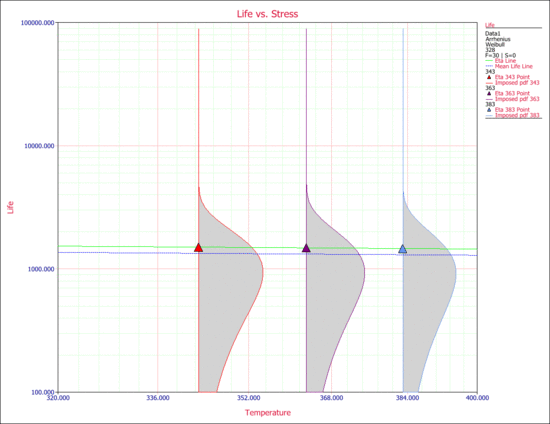
A small value for [math]\displaystyle{ B }[/math] is not the only indication for this behavior. One can also observe from the data that at all three stress levels, the times-to-failure are within the same range. Another way to observe this is by looking at the Arrhenius plot. The scale parameter, [math]\displaystyle{ \eta }[/math] , and the mean life are plotted next.
It can be seen that life ( [math]\displaystyle{ \eta }[/math] , and the mean life) is almost invariant with stress.
