Recurrent Event Data Analysis

Recurrent Event Data Analysis (RDA) is used in various applied fields such as reliability, medicine, social sciences, economics, business and criminology.

Whereas in life data analysis (LDA) it was assumed that events (failures) were independent and identically distributed (iid), there are many cases where events are dependent and not identically distributed (such as repairable system data) or where the analyst is interested in modeling the number of occurrences of events over time rather than the length of time prior to the first event, as in LDA.

Weibull++ provides both parametric and non-parametric approaches to analyze such data.

• The non-parametric approach is based on the well-known Mean Cumulative Function (MCF). The Weibull++ module for this type of analysis builds upon the work of Dr. Wayne Nelson, who has written extensively on the calculation and applications of MCF [31].

• The parametric approach is based on the General Renewal Process (GRP) model, which is particularly useful in understanding the effects of the repairs on the age of a system. Traditionally, the commonly used models for analyzing repairable systems data are the perfect renewal processes (PRP), which corresponds to perfect repairs, and the nonhomogeneous Poisson processes (NHPP), which corresponds to minimal repairs. However, most repair activities may realistically not result in such extreme situations but in a complicated intermediate one (general repair or imperfect repair/maintenance), which are well treated with the GRP model.

Non-Parametric Recurrent Event Data Analysis

Non-parametric RDA provides a non-parametric graphical estimate of the mean cumulative number or cost of recurrence per unit versus age. In the reliability field, the Mean Cumulative Function (MCF) can be used to: [31]

• Evaluate whether the population repair (or cost) rate increases or decreases with age (this is useful for product retirement and burn-in decisions).
• Estimate the average number or cost of repairs per unit during warranty or some time period.
• Compare two or more sets of data from different designs, production periods, maintenance policies, environments, operating conditions, etc.
• Predict future numbers and costs of repairs, such as the expected number of failures next month, quarter, or year.
• Reveal unexpected information and insight.

The Mean Cumulative Function (MCF)

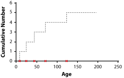
In a non-parametric analysis of recurrent event data, each population unit can be described by a cumulative history function for the cumulative number of recurrences. It is a staircase function that depicts the cumulative number of recurrences of a particular event, such as repairs over time. The figure below depicts a unit's cumulative history function.

The non-parametric model for a population of units is described as the population of cumulative history functions (curves). It is the population of all staircase functions of every unit in the population. At age t, the units have a distribution of their cumulative number of events. That is, a fraction of the population has accumulated 0 recurrences, another fraction has accumulated 1 recurrence, another fraction has accumulated 2 recurrences, etc. This distribution differs at different ages t , and has a mean M(t) called the mean cumulative function (MCF). The M(t) is the point-wise average of all population cumulative history functions (see figure below).

For the case of uncensored data, the mean cumulative function [math]\displaystyle{ M{{(t)}_{i}}\ }[/math] values at different recurrence ages t_i are estimated by calculating the average of the cumulative number of recurrences of events for each unit in the population at t_i . When the histories are censored, the following steps are applied.

1st Step - Order all ages:

Order all recurrence and censoring ages from smallest to largest. If a recurrence age for a unit is the same as its censoring (suspension) age, then the recurrence age goes first. If multiple units have a common recurrence or censoring age, then these units could be put in a certain order or be sorted randomly.

2nd Step - Calculate the number, r_i , of units that passed through age t_i :

[math]\displaystyle{ \begin{align} & {{r}_{i}}= & {{r}_{i-1}}\quad \quad \text{if }{{t}_{i}}\text{ is a recurrence age} \\ & {{r}_{i}}= & {{r}_{i-1}}-1\text{ if }{{t}_{i}}\text{ is a censoring age} \end{align} }[/math]

N is the total number of units and r₁ = N at the first observed age which could be a recurrence or suspension.

3rd Step - Calculate the MCF estimate, M*(t):

For each sample recurrence age t_i, calculate the mean cumulative function estimate as follows

[math]\displaystyle{ {{M}^{*}}({{t}_{i}})=\frac{1}{{{r}_{i}}}+{{M}^{*}}({{t}_{i-1}}) }[/math]

where [math]\displaystyle{ {{M}^{*}}(t)=\tfrac{1}{{{r}_{1}}} }[/math] at the earliest observed recurrence age, t₁ .

Confidence Limits for the MCF

Upper and lower confidence limits for [math]\displaystyle{ M({{t}_{i}}) }[/math] are:

[math]\displaystyle{ \begin{align} & {{M}_{U}}({{t}_{i}})= {{M}^{*}}({{t}_{i}}).{{e}^{\tfrac{{{K}_{\alpha }}.\sqrt{Var[{{M}^{*}}({{t}_{i}})]}}{{{M}^{*}}({{t}_{i}})}}} \\ & {{M}_{L}}({{t}_{i}})= \frac{{{M}^{*}}({{t}_{i}})}{{{e}^{\tfrac{{{K}_{\alpha }}.\sqrt{Var[{{M}^{*}}({{t}_{i}})]}}{{{M}^{*}}({{t}_{i}})}}}} \end{align} }[/math]

where [math]\displaystyle{ \alpha }[/math] ( [math]\displaystyle{ 50%\lt \alpha \lt 100% }[/math] ) is confidence level, [math]\displaystyle{ {{K}_{\alpha }} }[/math] is the [math]\displaystyle{ \alpha }[/math] standard normal percentile and [math]\displaystyle{ Var[{{M}^{*}}({{t}_{i}})] }[/math] is the variance of the MCF estimate at recurrence age [math]\displaystyle{ {{t}_{i}} }[/math] . The variance is calculated as follows:

[math]\displaystyle{ Var[{{M}^{*}}({{t}_{i}})]=Var[{{M}^{*}}({{t}_{i-1}})]+\frac{1}{r_{i}^{2}}\left[ \underset{j\in {{R}_{i}}}{\overset{}{\mathop \sum }}\,{{\left( {{d}_{ji}}-\frac{1}{{{r}_{i}}} \right)}^{2}} \right] }[/math]

where [math]\displaystyle{ {r}_{i} }[/math] is defined in the equation of the survivals, [math]\displaystyle{ {{R}_{i}} }[/math] is the set of the units that have not been suspended by [math]\displaystyle{ i }[/math] and [math]\displaystyle{ {{d}_{ji}} }[/math] is defined as follows:

[math]\displaystyle{ \begin{align} & {{d}_{ji}}= 1\text{ if the }{{j}^{\text{th }}}\text{unit had an event recurrence at age }{{t}_{i}} \\ & {{d}_{ji}}= 0\text{ if the }{{j}^{\text{th }}}\text{unit did not have an event reoccur at age }{{t}_{i}} \end{align} }[/math]

Example: Mean Cumulative Function

A health care company maintains five identical pieces of equipment used by a hospital. When a piece of equipment fails, the company sends a crew to repair it. The following table gives the failure and censoring ages for each machine, where the + sign indicates a censoring age.

[math]\displaystyle{ \begin{matrix} Equipment ID & Months \\ \text{1} & \text{5, 10 , 15, 17+} \\ \text{2} & \text{6, 13, 17, 19+} \\ \text{3} & \text{12, 20, 25, 26+} \\ \text{4} & \text{13, 15, 24+} \\ \text{5} & \text{16, 22, 25, 28+} \\ \end{matrix} }[/math]

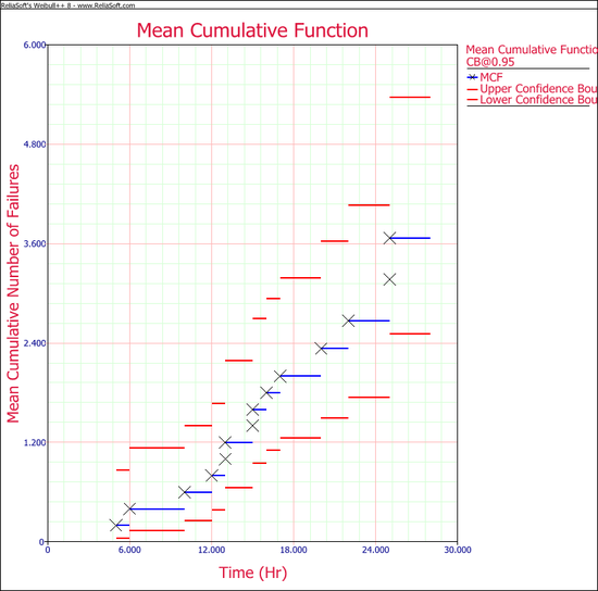
Estimate the MCF values, with 95% confidence bounds.

Solution

The MCF estimates are obtained as follows:

[math]\displaystyle{ \begin{matrix} ID & Months ({{t}_{i}}) & State & {{r}_{i}} & 1/{{r}_{i}} & {{M}^{*}}({{t}_{i}}) \\ \text{1} & \text{5} & \text{F} & \text{5} & \text{0}\text{.20} & \text{0}\text{.20} \\ \text{2} & \text{6} & \text{F} & \text{5} & \text{0}\text{.20} & \text{0}\text{.20 + 0}\text{.20 = 0}\text{.40} \\ \text{1} & \text{10} & \text{F} & \text{5} & \text{0}\text{.20} & \text{0}\text{.40 + 0}\text{.20 = 0}\text{.60} \\ \text{3} & \text{12} & \text{F} & \text{5} & \text{0}\text{.20} & \text{0}\text{.60 + 0}\text{.20 = 0}\text{.80} \\ \text{2} & \text{13} & \text{F} & \text{5} & \text{0}\text{.20} & \text{0}\text{.80+0}\text{.20 =1}\text{.00} \\ \text{4} & \text{13} & \text{F} & \text{5} & \text{0}\text{.20} & \text{1}\text{.00 + 0}\text{.20 = 1}\text{.20} \\ \text{1} & \text{15} & \text{F} & \text{5} & \text{0}\text{.20} & \text{1}\text{.20 + 0}\text{.20 =1}\text{.40} \\ \text{4} & \text{15} & \text{F} & \text{5} & \text{0}\text{.20} & \text{1}\text{.40 + 0}\text{.20 = 1}\text{.60} \\ \text{5} & \text{16} & \text{F} & \text{5} & \text{0}\text{.20} & \text{1}\text{.60 + 0}\text{.20 = 1}\text{.80} \\ \text{2} & \text{17} & \text{F} & \text{5} & \text{0}\text{.20} & \text{1}\text{.80 + 0}\text{.20 = 2}\text{.0} \\ \text{1} & \text{17} & \text{S} & \text{4} & {} & {} \\ \text{2} & \text{19} & \text{S} & \text{3} & {} & {} \\ \text{3} & \text{20} & \text{F} & \text{3} & \text{0}\text{.33} & \text{2}\text{.00 + 0}\text{.33 = 2}\text{.33} \\ \text{5} & \text{22} & \text{F} & \text{3} & \text{0}\text{.33} & \text{2}\text{.33 + 0}\text{.33 = 2}\text{.66} \\ \text{4} & \text{24} & \text{S} & \text{2} & {} & {} \\ \text{3} & \text{25} & \text{F} & \text{2} & \text{0}\text{.50} & \text{2}\text{.66 + 0}\text{.50 = 3}\text{.16} \\ \text{5} & \text{25} & \text{F} & \text{2} & \text{0}\text{.50} & \text{3}\text{.16 + 0}\text{.50 = 3}\text{.66} \\ \text{3} & \text{26} & \text{S} & \text{1} & {} & {} \\ \text{5} & \text{28} & \text{S} & \text{0} & {} & {} \\ \end{matrix} }[/math]

Using the MCF variance equation, the following table of variance values can be obtained:

ID	Months	State	ri	V'a'ri
1	5	F	5	[math]\displaystyle{ (\tfrac{1}{5})^2[(1-\tfrac{1}{5})^2+4(0-\tfrac{1}{5})^2]=0.032 }[/math]
2	6	F	5	[math]\displaystyle{ 0.032+(\tfrac{1}{5})^2[(1-\tfrac{1}{5})^2+4(0-\tfrac{1}{5})^2]=0.064 }[/math]
1	10	F	5	[math]\displaystyle{ 0.064+(\tfrac{1}{5})^2[(1-\tfrac{1}{5})^2+4(0-\tfrac{1}{5})^2]=0.096 }[/math]
3	12	F	5	[math]\displaystyle{ 0.096+(\tfrac{1}{5})^2[(1-\tfrac{1}{5})^2+4(0-\tfrac{1}{5})^2]=0.128 }[/math]
2	13	F	5	[math]\displaystyle{ 0.128+(\tfrac{1}{5})^2[(1-\tfrac{1}{5})^2+4(0-\tfrac{1}{5})^2]=0.160 }[/math]
4	13	F	5	[math]\displaystyle{ 0.160+(\tfrac{1}{5})^2[(1-\tfrac{1}{5})^2+4(0-\tfrac{1}{5})^2]=0.192 }[/math]
1	15	F	5	[math]\displaystyle{ 0.192+(\tfrac{1}{5})^2[(1-\tfrac{1}{5})^2+4(0-\tfrac{1}{5})^2]=0.224 }[/math]
4	15	F	5	[math]\displaystyle{ 0.224+(\tfrac{1}{5})^2[(1-\tfrac{1}{5})^2+4(0-\tfrac{1}{5})^2]=0.256 }[/math]
5	16	F	5	[math]\displaystyle{ 0.256+(\tfrac{1}{5})^2[3(0-\tfrac{1}{5})^2+2(1-\tfrac{1}{5})^2]=0.288 }[/math]
2	17	F	5	[math]\displaystyle{ 0.288+(\tfrac{1}{5})^2[(1-\tfrac{1}{5})^2+4(0-\tfrac{1}{5})^2]=0.320 }[/math]
1	17	S	4
2	19	S	3
3	20	F	3	[math]\displaystyle{ 0.320+(\tfrac{1}{5})^2[(1-\tfrac{1}{5})^2+2(0-\tfrac{1}{5})^2]=0.394 }[/math]
5	22	F	3	[math]\displaystyle{ 0.394+(\tfrac{1}{5})^2[2(0-\tfrac{1}{5})^2+4(1-\tfrac{1}{5})^2]=0.468 }[/math]
4	24	S	2
3	25	F	2	[math]\displaystyle{ 0.468+(\tfrac{1}{5})^2[(1-\tfrac{1}{5})^2+4(0-\tfrac{1}{5})^2]=0.593 }[/math]
5	25	F	2	[math]\displaystyle{ 0.580+(\tfrac{1}{5})^2[(0-\tfrac{1}{5})^2+4(1-\tfrac{1}{5})^2]=0.718 }[/math]
3	26	S	1
5	28	S	0

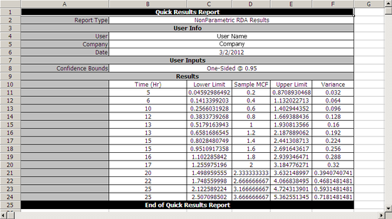
Using the equation for the MCF bounds and K₅ = 1.644 for a 95% confidence level, the confidence bounds can be obtained as follows:

[math]\displaystyle{ \begin{matrix} ID & Months & State & MC{{F}_{i}} & Va{{r}_{i}} & MC{{F}_{{{L}_{i}}}} & MC{{F}_{{{U}_{i}}}} \\ \text{1} & \text{5} & \text{F} & \text{0}\text{.20} & \text{0}\text{.032} & 0.0459 & 0.8709 \\ \text{2} & \text{6} & \text{F} & \text{0}\text{.40} & \text{0}\text{.064} & 0.1413 & 1.1320 \\ \text{1} & \text{10} & \text{F} & \text{0}\text{.60} & \text{0}\text{.096} & 0.2566 & 1.4029 \\ \text{3} & \text{12} & \text{F} & \text{0}\text{.80} & \text{0}\text{.128} & 0.3834 & 1.6694 \\ \text{2} & \text{13} & \text{F} & \text{1}\text{.00} & \text{0}\text{.160} & 0.5179 & 1.9308 \\ \text{4} & \text{13} & \text{F} & \text{1}\text{.20} & \text{0}\text{.192} & 0.6582 & 2.1879 \\ \text{1} & \text{15} & \text{F} & \text{1}\text{.40} & \text{0}\text{.224} & 0.8028 & 2.4413 \\ \text{4} & \text{15} & \text{F} & \text{1}\text{.60} & \text{0}\text{.256} & 0.9511 & 2.6916 \\ \text{5} & \text{16} & \text{F} & \text{1}\text{.80} & \text{0}\text{.288} & 1.1023 & 2.9393 \\ \text{2} & \text{17} & \text{F} & \text{2}\text{.0} & \text{0}\text{.320} & 1.2560 & 3.1848 \\ \text{1} & \text{17} & \text{S} & {} & {} & {} & {} \\ \text{2} & \text{19} & \text{S} & {} & {} & {} & {} \\ \text{3} & \text{20} & \text{F} & \text{2}\text{.33} & \text{0}\text{.394} & 1.4990 & 3.6321 \\ \text{5} & \text{22} & \text{F} & \text{2}\text{.66} & \text{0}\text{.468} & 1.7486 & 4.0668 \\ \text{4} & \text{24} & \text{S} & {} & {} & {} & {} \\ \text{3} & \text{25} & \text{F} & \text{3}\text{.16} & \text{0}\text{.593} & 2.1226 & 4.7243 \\ \text{5} & \text{25} & \text{F} & \text{3}\text{.66} & \text{0}\text{.718} & 2.5071 & 5.3626 \\ \text{3} & \text{26} & \text{S} & {} & {} & {} & {} \\ \text{5} & \text{28} & \text{S} & {} & {} & {} & {} \\ \end{matrix} }[/math]

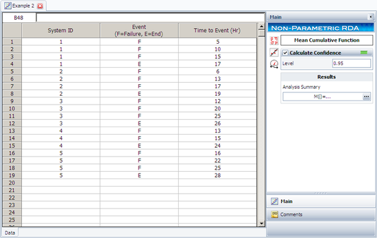
The analysis presented in this example can be performed automatically in Weibull++'s non-parametric RDA folio, as shown next.

Note: In the folio above, the F refers to failures and E refers to suspensions (or censoring ages). The results, with calculated MCF values and upper and lower 95% confidence limits, are shown next along with the graphical plot.

Parametric Recurrent Event Data Analysis

Weibull++'s parametric RDA folio is a tool for modeling recurrent event data. It can capture the trend, estimate the rate and predict the total number of recurrences. The failure and repair data of a repairable system can be treated as one type of recurrence data. Past and current repairs may affect the future failure process. For most recurrent events, time (distance, cycles, etc.) is a key factor. With time, the recurrence rate may remain constant, increase or decrease. For other recurrent events, not only the time, but also the number of events can affect the recurrence process (e.g., the debugging process in software development). The parametric analysis approach utilizes the General Renewal Process (GRP) model [28]. In this model, the repair time is assumed to be negligible so that the processes can be viewed as point processes. This model provides a way to describe the rate of occurrence of events over time, such as in the case of data obtained from a repairable system. This model is particularly useful in modeling the failure behavior of a specific system and understanding the effects of the repairs on the age of that system. For example, consider a system that is repaired after a failure, where the repair does not bring the system to an as-good-as-new or an as-bad-as-old condition. In other words, the system is partially rejuvenated after the repair. Traditionally, in as-bad-as-old repairs, also known as minimal repairs, the failure data from such a system would have been modeled using a homogeneous or non-homogeneous Poisson process (NHPP). On rare occasions, a Weibull distribution has been used as well in cases where the system is almost as-good-as-new after the repair, also known as a perfect renewal process (PRP). However, for the intermediate states after the repair, there has not been a commercially available model, even though many models have been proposed in literature. In Weibull++, the GRP model provides the capability to model systems with partial renewal (general repair or imperfect repair/maintenance) and allows for a variety of predictions such as reliability, expected failures, etc.

The GRP Model

In this model, the concept of virtual age is introduced. Let [math]\displaystyle{ {{t}_{1}},{{t}_{2}},\cdots ,{{t}_{n}} }[/math] represent the successive failure times and let [math]\displaystyle{ {{x}_{1}},{{x}_{2}},\cdots ,{{x}_{n}} }[/math] represent the time between failures ( [math]\displaystyle{ {{t}_{i}}=\sum_{j=1}^{i}{{x}_{j}}) }[/math] . Assume that after each event, actions are taken to improve the system performance. Let q be the action effectiveness factor. There are two GRP models:

Type I:

v_i = v_{i − 1} + q''x = qt_i

Type II:

[math]\displaystyle{ {{v}_{i}}=q({{v}_{i-1}}+{{x}_{i}})={{q}^{i}}{{x}_{1}}+{{q}^{i-1}}{{x}_{2}}+\cdots +{{x}_{i}} }[/math]

where v_i is the virtual age of the system right after i th repair. The Type I model assumes that the i th repair cannot remove the damage incurred before the ith failure. It can only reduce the additional age x_i to q'x_i . The Type II model assumes that at the i th repair, the virtual age has been accumulated to v_{i − 1} + x_i . The i th repair will remove the cumulative damage from both current and previous failures by reducing the virtual age to q(v_{i − 1} + x_i) .

The power law function is used to model the rate of recurrence, which is:

λ(t) = λβt^{β − 1}

The conditional pdf is:

[math]\displaystyle{ f({{t}_{i}}|{{t}_{i-1}})=\lambda \beta {{({{x}_{i}}+{{v}_{i-1}})}^{\beta -1}}{{e}^{-\lambda \left[ {{\left( {{x}_{i}}+{{v}_{i-1}} \right)}^{\beta }}-v_{i-1}^{\beta } \right]}} }[/math]

MLE method is used to estimate the model parameters. The log likelihood function is [28]:

[math]\displaystyle{ \begin{align} & \ln (L)= n(\ln \lambda +\ln \beta )-\lambda \left[ {{\left( T-{{t}_{n}}+{{v}_{n}} \right)}^{\beta }}-v_{n}^{\beta } \right] \\ & -\lambda \underset{i=1}{\overset{n}{\mathop \sum }}\,\left[ {{\left( {{x}_{i}}+{{v}_{i-1}} \right)}^{\beta }}-v_{i}^{\beta } \right]+(\beta -1)\underset{i=1}{\overset{n}{\mathop \sum }}\,\ln ({{x}_{i}}+{{v}_{i-1}}) \end{align} }[/math]

where n is the total number of events during the entire observation period. T is the stop time of the observation. T = t_n if the observation stops right after the last event.

Confidence Bounds

In general, in order to obtain the virtual age, the exact occurrence time of each event (failure) should be available (see equations for Type I and Type II models). However, the times are unknown until the corresponding events occur. For this reason, there are no closed-form expressions for total failure number and failure intensity, which are functions of failure times and virtual age. Therefore, in Weibull++, a Monte Carlo simulation is used to predict values of virtual time, failure number, MTBF and failure rate. The approximate confidence bounds obtained from simulation are provided. The uncertainty of model parameters is also considered in the bounds.

Bounds on Cumulative Failure (Event) Numbers

The variance of the cumulative failure number N(t) is:

[math]\displaystyle{ Var[N(t)]=Var\left[ E(N(t)|\lambda ,\beta ,q) \right]+E\left[ Var(N(t)|\lambda ,\beta ,q) \right] }[/math]

The first term accounts for the uncertainty of the parameter estimation. The second term considers the uncertainty caused by the renewal process even when model parameters are fixed. However, unless q = 1 , [math]\displaystyle{ Var\left[ E(N(t)|\lambda ,\beta ,q) \right] }[/math] cannot be calculated because E(N(t)) cannot be expressed as a closed-form function of λ,β, and q . In order to consider the uncertainty of the parameter estimation, [math]\displaystyle{ Var\left[ E(N(t)|\lambda ,\beta ,q) \right] }[/math] is approximated by:

[math]\displaystyle{ Var\left[ E(N(t)|\lambda ,\beta ,q) \right]=Var[E(N({{v}_{t}})|\lambda ,\beta )]=Var[\lambda v_{t}^{\beta }] }[/math]

where v_t is the expected virtual age at time t and [math]\displaystyle{ Var[\lambda v_{t}^{\beta }] }[/math] is::

[math]\displaystyle{ \begin{align} & Var[\lambda v_{t}^{\beta }]= & {{\left( \frac{\partial (\lambda v_{t}^{\beta })}{\partial \beta } \right)}^{2}}Var(\hat{\beta })+{{\left( \frac{\partial (\lambda v_{t}^{\beta })}{\partial \lambda } \right)}^{2}}Var(\hat{\lambda }) \\ & +2\frac{\partial (\lambda v_{t}^{\beta })}{\partial \beta }\frac{\partial (\lambda v_{t}^{\beta })}{\partial \lambda }Cov(\hat{\beta },\hat{\lambda }) \end{align} }[/math]

By conducting this approximation, the uncertainty of λ and β are considered. The value of v_t and the value of the second term in the equation for the variance of number of failures are obtained through the Monte Carlo simulation using parameters [math]\displaystyle{ \hat{\lambda },\hat{\beta },\hat{q}, }[/math] which are the ML estimators. The same simulation is used to estimate the cumulative number of failures [math]\displaystyle{ \hat{N}(t)=E(N(t)|\hat{\lambda },\hat{\beta },\hat{q}) }[/math] .

Once the variance and the expected value of N(t) have been obtained, the bounds can be calculated by assuming that N(t) is lognormally distributed as:

[math]\displaystyle{ \frac{\ln N(t)-\ln \hat{N}(t)}{\sqrt{Var(\ln N(t))}}\tilde{\ }N(0,1) }[/math]

The upper and lower bounds for a given confidence level α can be calculated by:

[math]\displaystyle{ N{{(t)}_{U,L}}=\hat{N}(t){{e}^{\pm {{z}_{a}}\sqrt{Var(N(t))}/\hat{N}(t)}} }[/math]

where z_a is the standard normal distribution.

If N(t) is assumed to be normally distributed, the bounds can be calculated by:

[math]\displaystyle{ N{{(t)}_{U}}=\hat{N}(t)+{{z}_{a}}\sqrt{Var(N(t))} }[/math]

[math]\displaystyle{ N{{(t)}_{L}}=\hat{N}(t)-{{z}_{a}}\sqrt{Var(N(t))} }[/math]

In Weibull++, the N(t)_U is the smaller of the upper bounds obtained from lognormal and normal distribution appoximation. The N(t)_L is set to the largest of the lower bounds obtained from lognormal and normal distribution appoximation. This combined method can prevent the out-of-range values of bounds for some small t values.

Bounds of Cumulative Failure Intensity and MTBF

For a given time t , the expected value of cumulative MTBF m_c(t) and cumulative failure intensity λ_c(t) can be calculated using the following equations:

[math]\displaystyle{ {{\hat{\lambda }}_{c}}(t)=\frac{\hat{N}(t)}{t};{{\hat{m}}_{c}}(t)=\frac{t}{\hat{N}(t)} }[/math]

The bounds can be easily obtained from the corresponding bounds of N(t).

[math]\displaystyle{ \begin{align} & {{{\hat{\lambda }}}_{c}}{{(t)}_{L}}= & \frac{\hat{N}{{(t)}_{L}}}{t};\text{ }{{{\hat{\lambda }}}_{c}}{{(t)}_{L}}=\frac{\hat{N}{{(t)}_{L}}}{t};\text{ } \\ & {{{\hat{m}}}_{c}}{{(t)}_{L}}= & \frac{t}{\hat{N}{{(t)}_{U}}};\text{ }{{{\hat{m}}}_{c}}{{(t)}_{U}}=\frac{t}{\hat{N}{{(t)}_{L}}} \end{align} }[/math]

Bounds on Instantaneous Failure Intensity and MTBF

The instantaneous failure intensity is given by:

[math]\displaystyle{ {{\lambda }_{i}}(t)=\lambda \beta v_{t}^{\beta -1} }[/math]

where v_t is the virtual age at time t. When [math]\displaystyle{ q\ne 1, }[/math] it is obtained from simulation. When q = 1 , v_t = t from model Type I and Type II.

The variance of instantaneous failure intensity can be calculated by:

[math]\displaystyle{ \begin{align} & Var({{\lambda }_{i}}(t))= {{\left( \frac{\partial {{\lambda }_{i}}(t)}{\partial \beta } \right)}^{2}}Var(\hat{\beta })+{{\left( \frac{\partial {{\lambda }_{i}}(t)}{\partial \lambda } \right)}^{2}}Var(\hat{\lambda }) \\ & +2\frac{\partial {{\lambda }_{i}}(t)}{\partial \beta }\frac{\partial {{\lambda }_{i}}(t)}{\partial \lambda }Cov(\hat{\beta },\hat{\lambda })+{{\left( \frac{\partial {{\lambda }_{i}}(t)}{\partial v(t)} \right)}^{2}}Var({{{\hat{v}}}_{t}}) \end{align} }[/math]

The expected value and variance of v_t are obtained from the Monte Carlo simulation with parameters [math]\displaystyle{ \hat{\lambda },\hat{\beta },\hat{q}. }[/math] Because of the simulation accuracy and the convergence problem in calculation of [math]\displaystyle{ Var(\hat{\beta }),Var(\hat{\lambda }) }[/math] and [math]\displaystyle{ Cov(\hat{\beta },\hat{\lambda }), }[/math] V'a'r(λ_i(t)) can be a negative value at some time points. When this case happens, the bounds of instantaneous failure intensity are not provided.

Once the variance and the expected value of λ_i(t) are obtained, the bounds can be calculated by assuming that  λ_i(t) is lognormally distributed as:

[math]\displaystyle{ \frac{\ln {{\lambda }_{i}}(t)-\ln {{{\hat{\lambda }}}_{i}}(t)}{\sqrt{Var(\ln {{\lambda }_{i}}(t))}}\tilde{\ }N(0,1) }[/math]

The upper and lower bounds for a given confidence level α can be calculated by:

[math]\displaystyle{ {{\lambda }_{i}}(t)={{\hat{\lambda }}_{i}}(t){{e}^{\pm {{z}_{a}}\sqrt{Var({{\lambda }_{i}}(t))}/{{{\hat{\lambda }}}_{i}}(t)}} }[/math]

where z_a is the standard normal distribution.

If λ_i(t) is assumed to be normally distributed, the bounds can be calculated by:

[math]\displaystyle{ {{\lambda }_{i}}{{(t)}_{U}}={{\hat{\lambda }}_{i}}(t)+{{z}_{a}}\sqrt{Var(N(t))} }[/math]

[math]\displaystyle{ {{\lambda }_{i}}{{(t)}_{L}}={{\hat{\lambda }}_{i}}(t)-{{z}_{a}}\sqrt{Var(N(t))} }[/math]

In Weibull++, λ_i(t)_U is set to the smaller of the two upper bounds obtained from the above lognormal and normal distribution appoximation. λ_i(t)_L is set to the largest of the two lower bounds obtained from the above lognormal and normal distribution appoximation. This combination method can prevent the out of range values of bounds when t values are small.

For a given time t , the expected value of cumulative MTBF m_i(t) is:

[math]\displaystyle{ {{\hat{m}}_{i}}(t)=\frac{1}{{{{\hat{\lambda }}}_{i}}(t)}\text{ } }[/math]

The upper and lower bounds can be easily obtained from the corresponding bounds of λ_i(t):

[math]\displaystyle{ {{\hat{m}}_{i}}{{(t)}_{U}}=\frac{1}{{{{\hat{\lambda }}}_{i}}{{(t)}_{L}}} }[/math]

[math]\displaystyle{ {{\hat{m}}_{i}}{{(t)}_{L}}=\frac{1}{{{{\hat{\lambda }}}_{i}}{{(t)}_{U}}} }[/math]

Bounds on Conditional Reliability

Given mission start time t₀ and mission time T , the conditional reliability can be calculated by:

[math]\displaystyle{ R(T|{{t}_{0}})=\frac{R(T+{{v}_{0}})}{R({{v}_{0}})}={{e}^{-\lambda [{{({{v}_{0}}+T)}^{\beta }}-{{v}_{0}}]}} }[/math]

v₀ is the virtual age corresponding to time t₀ . The expected value and the variance of v₀ are obtained from Monte Carlo simulation. The variance of the conditional reliability R(T | t₀) is:

[math]\displaystyle{ \begin{align} & Var(R)= {{\left( \frac{\partial R}{\partial \beta } \right)}^{2}}Var(\hat{\beta })+{{\left( \frac{\partial R}{\partial \lambda } \right)}^{2}}Var(\hat{\lambda }) \\ & +2\frac{\partial R}{\partial \beta }\frac{\partial R}{\partial \lambda }Cov(\hat{\beta },\hat{\lambda })+{{\left( \frac{\partial R}{\partial {{v}_{0}}} \right)}^{2}}Var({{{\hat{v}}}_{0}}) \end{align} }[/math]

Because of the simulation accuracy and the convergence problem in calculation of [math]\displaystyle{ Var(\hat{\beta }),Var(\hat{\lambda }) }[/math] and [math]\displaystyle{ Cov(\hat{\beta },\hat{\lambda }), }[/math] V'a'r(R) can be a negative value at some time points. When this case happens, the bounds are not provided.

The bounds are based on:

[math]\displaystyle{ \log \text{it}(\hat{R}(T))\tilde{\ }N(0,1) }[/math]

[math]\displaystyle{ \log \text{it}(\hat{R}(T))=\ln \left\{ \frac{\hat{R}(T)}{1-\hat{R}(T)} \right\} }[/math]

The confidence bounds on reliability are given by:

[math]\displaystyle{ R=\frac{{\hat{R}}}{\hat{R}+(1-\hat{R}){{e}^{\pm \sqrt{Var(R)}/[\hat{R}(1-\hat{R})]}}} }[/math]

It will be compared with the bounds obtained from:

[math]\displaystyle{ R=\hat{R}{{e}^{\pm {{z}_{a}}\sqrt{Var(R)}/\hat{R}}} }[/math]

The smaller of the two upper bounds will be the final upper bound and the larger of the two lower bounds will be the final lower bound.

Example: Air Condition Unit

The following table gives the failure times for the air conditioning unit of an aircraft. The observation ended by the time the last failure occurred, as discussed in Cox [3].

[math]\displaystyle{ \begin{matrix} \text{50} & \text{329} & \text{811} & \text{991} & \text{1489} \\ \text{94} & \text{332} & \text{899} & \text{1013} & \text{1512} \\ \text{196} & \text{347} & \text{945} & \text{1152} & \text{1525} \\ \text{268} & \text{544} & \text{950} & \text{1362} & \text{1539} \\ \text{290} & \text{732} & \text{955} & \text{1459} & {} \\ \end{matrix}\,\! }[/math]

1. Estimate the GRP model parameters using the Type I virtual age option.

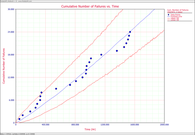
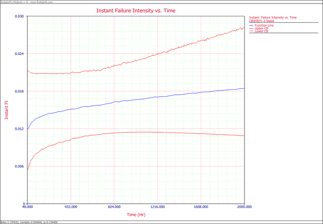
2. Plot the failure number and instantaneous failure intensity vs. time with 90% two-sided confidence bounds.

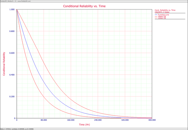
3. Plot the conditional reliability vs. time with 90% two-sided confidence bounds. The mission start time is 40 and mission time is varying.

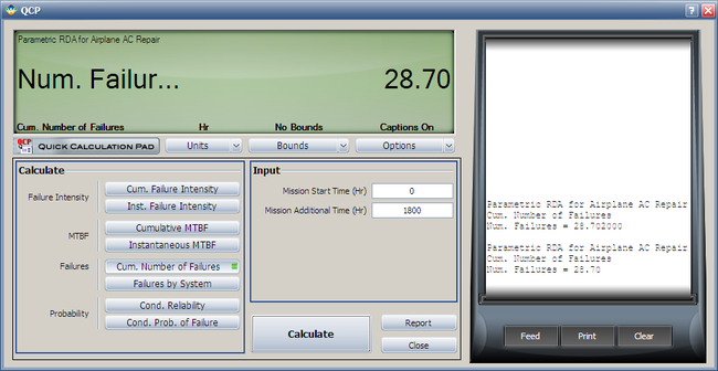
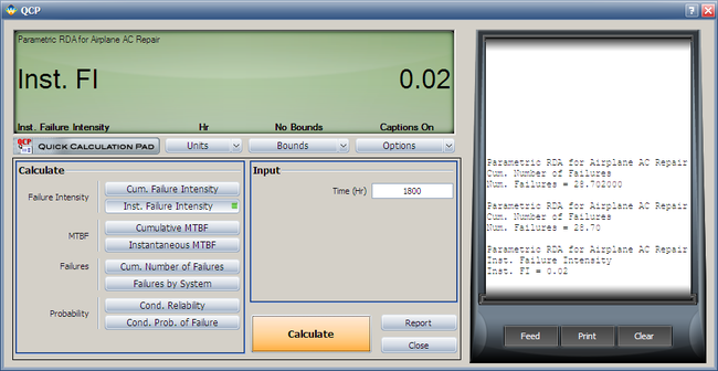
4. Using the QCP, calculate the expected failure number and expected instantaneous failure intensity by time 1800.

Solution

Enter the data into a parametric RDA folio in Weibull++. On the control panel, select the 3 parameters option and the Type I setting. Keep the default simulation settings. Click Calculate.

1. The estimated parameters are [math]\displaystyle{ \hat{\beta }=1.1976\,\! }[/math], [math]\displaystyle{ \hat{\lambda }=4.94E-03\,\! }[/math], [math]\displaystyle{ \hat{q}=0.1344\,\! }[/math].

2. The following plots show the cumulative number of failures and instantaneous failure intensity, respectively.

3. The following plot shows the conditional reliability.

4. Using the QCP, the failure number and instantaneous failure intensity are: