Template:Example: Normal Distribution MLE: Difference between revisions
Lisa Hacker (talk | contribs) No edit summary |
No edit summary |
||
| Line 6: | Line 6: | ||
In this example we have non-grouped data without suspensions and without interval data. The partial derivatives of the normal log-likelihood function, <math>\Lambda ,</math> are given by: | In this example we have non-grouped data without suspensions and without interval data. The partial derivatives of the normal log-likelihood function, <math>\Lambda ,</math> are given by: | ||
::<math>\begin{align} | ::<math>\begin{align} | ||
| Line 12: | Line 11: | ||
\frac{\partial \Lambda }{\partial \sigma }= & \underset{i=1}{\overset{14}{\mathop \sum }}\,\left( \frac{{{t}_{i}}-\mu }{{{\sigma }^{3}}}-\frac{1}{\sigma } \right)=0 | \frac{\partial \Lambda }{\partial \sigma }= & \underset{i=1}{\overset{14}{\mathop \sum }}\,\left( \frac{{{t}_{i}}-\mu }{{{\sigma }^{3}}}-\frac{1}{\sigma } \right)=0 | ||
\end{align}</math> | \end{align}</math> | ||
(The derivations of these equations are presented in [[Appendix:_Log-Likelihood_Equations|an appendix]].) Substituting the values of <math>{{t}_{i}}</math> and solving the above system simultaneously, we get <math>\widehat{\sigma }=29.58</math> hours <math>,</math> <math>\widehat{\mu }=45</math> hours <math>.</math> | (The derivations of these equations are presented in [[Appendix:_Log-Likelihood_Equations|an appendix]].) Substituting the values of <math>{{t}_{i}}</math> and solving the above system simultaneously, we get <math>\widehat{\sigma }=29.58</math> hours <math>,</math> <math>\widehat{\mu }=45</math> hours <math>.</math> | ||
| Line 23: | Line 21: | ||
\widehat{Cov}\left( \widehat{\mu },\widehat{\sigma } \right)=0.0000 & {} & \widehat{Var}\left( \widehat{\sigma } \right)=31.2500 \\ | \widehat{Cov}\left( \widehat{\mu },\widehat{\sigma } \right)=0.0000 & {} & \widehat{Var}\left( \widehat{\sigma } \right)=31.2500 \\ | ||
\end{matrix} \right]</math> | \end{matrix} \right]</math> | ||
Using Weibull++ , the MLE method can be selected from the Set Analysis page. | Using Weibull++ , the MLE method can be selected from the Set Analysis page. | ||
[[Image:Normal MLE Setting.png | [[Image:Normal MLE Setting.png|center|550px| ]] | ||
The plot of the solution for this example is shown next. | The plot of the solution for this example is shown next. | ||
[[Image:Normal MLE Plot.png | [[Image:Normal MLE Plot.png|center|550px| ]] | ||
Revision as of 02:39, 8 August 2012
Normal Distribution MLE Example
Using the data of Example 2 and assuming a normal distribution, estimate the parameters using the MLE method.
Solution
In this example we have non-grouped data without suspensions and without interval data. The partial derivatives of the normal log-likelihood function, [math]\displaystyle{ \Lambda , }[/math] are given by:
- [math]\displaystyle{ \begin{align} \frac{\partial \Lambda }{\partial \mu }= & \frac{1}{{{\sigma }^{2}}}\underset{i=1}{\overset{14}{\mathop \sum }}\,({{t}_{i}}-\mu )=0 \\ \frac{\partial \Lambda }{\partial \sigma }= & \underset{i=1}{\overset{14}{\mathop \sum }}\,\left( \frac{{{t}_{i}}-\mu }{{{\sigma }^{3}}}-\frac{1}{\sigma } \right)=0 \end{align} }[/math]
(The derivations of these equations are presented in an appendix.) Substituting the values of [math]\displaystyle{ {{t}_{i}} }[/math] and solving the above system simultaneously, we get [math]\displaystyle{ \widehat{\sigma }=29.58 }[/math] hours [math]\displaystyle{ , }[/math] [math]\displaystyle{ \widehat{\mu }=45 }[/math] hours [math]\displaystyle{ . }[/math]
The Fisher matrix is:
- [math]\displaystyle{ \left[ \begin{matrix} \widehat{Var}\left( \widehat{\mu } \right)=62.5000 & {} & \widehat{Cov}\left( \widehat{\mu },\widehat{\sigma } \right)=0.0000 \\ {} & {} & {} \\ \widehat{Cov}\left( \widehat{\mu },\widehat{\sigma } \right)=0.0000 & {} & \widehat{Var}\left( \widehat{\sigma } \right)=31.2500 \\ \end{matrix} \right] }[/math]
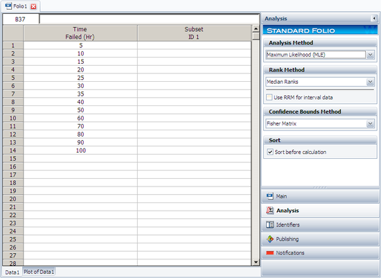
Using Weibull++ , the MLE method can be selected from the Set Analysis page.
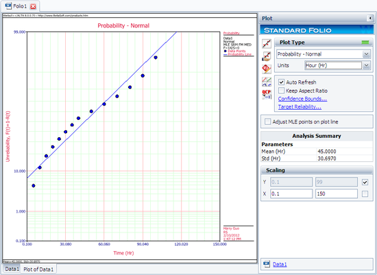
The plot of the solution for this example is shown next.

