Template:Mean cumulative function for recurrence data

The Mean Cumulative Function (MCF) for Recurrent Event Data Analysis

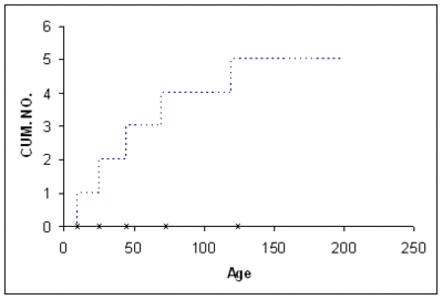
In a non-parametric analysis of recurrent event data, each population unit can be described by a cumulative history function for the cumulative number of recurrences. It is a staircase function that depicts the cumulative number of recurrences of a particular event, such as repairs over time. The figure below depicts a unit's cumulative history function.

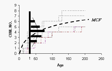
The non-parametric model for a population of units is described as the population of cumulative history functions (curves). It is the population of all staircase functions of every unit in the population. At age t, the units have a distribution of their cumulative number of events. That is, a fraction of the population has accumulated 0 recurrences, another fraction has accumulated 1 recurrence, another fraction has accumulated 2 recurrences, etc. This distribution differs at different ages t , and has a mean M(t) called the mean cumulative function (MCF). The M(t) is the point-wise average of all population cumulative history functions (see figure below).

For the case of uncensored data, the mean cumulative function [math]\displaystyle{ M{{(t)}_{i}}\ }[/math] values at different recurrence ages t_i are estimated by calculating the average of the cumulative number of recurrences of events for each unit in the population at t_i . When the histories are censored, the following steps are applied.

1st Step - Order all ages:

Order all recurrence and censoring ages from smallest to largest. If a recurrence age for a unit is the same as its censoring (suspension) age, then the recurrence age goes first. If multiple units have a common recurrence or censoring age, then these units could be put in a certain order or be sorted randomly.

2nd Step - Calculate the number, r_i , of units that passed through age t_i :

[math]\displaystyle{ \begin{align} & {{r}_{i}}= & {{r}_{i-1}}\quad \quad \text{if }{{t}_{i}}\text{ is a recurrence age} \\ & {{r}_{i}}= & {{r}_{i-1}}-1\text{ if }{{t}_{i}}\text{ is a censoring age} \end{align} }[/math]

N is the total number of units and r₁ = N at the first observed age which could be a recurrence or suspension.

3rd Step - Calculate the M<span class="texhtml" />C'F'estimate, <span class="texhtml" />:For each sample recurrence age <span class="texhtml" />calculate the mean cumulative function estimate as follows:M^* (t)t,

[math]\displaystyle{ {{M}^{*}}({{t}_{i}})=\frac{1}{{{r}_{i}}}+{{M}^{*}}({{t}_{i-1}}) }[/math]

where [math]\displaystyle{ {{M}^{*}}(t)=\tfrac{1}{{{r}_{1}}} }[/math] at the earliest observed recurrence age, t₁ .

Example 1: A health care company maintains five identical pieces of equipment used by a hospital. When a piece of equipment fails, the company sends a crew to repair it. The following table gives the failure and censoring ages for each machine, where the + sign indicates a censoring age.

[math]\displaystyle{ \begin{matrix} Equipment ID & Months \\ \text{1} & \text{5, 10 , 15, 17+} \\ \text{2} & \text{6, 13, 17, 19+} \\ \text{3} & \text{12, 20, 25, 26+} \\ \text{4} & \text{13, 15, 24+} \\ \text{5} & \text{16, 22, 25, 28+} \\ \end{matrix}\,\! }[/math]

Estimate the MCF values, with 95% confidence bounds.

Solution

The MCF estimates are obtained as follows:

[math]\displaystyle{ \begin{matrix} ID & Months ({{t}_{i}}) & State & {{r}_{i}} & 1/{{r}_{i}} & {{M}^{*}}({{t}_{i}}) \\ \text{1} & \text{5} & \text{F} & \text{5} & \text{0}\text{.20} & \text{0}\text{.20} \\ \text{2} & \text{6} & \text{F} & \text{5} & \text{0}\text{.20} & \text{0}\text{.20 + 0}\text{.20 = 0}\text{.40} \\ \text{1} & \text{10} & \text{F} & \text{5} & \text{0}\text{.20} & \text{0}\text{.40 + 0}\text{.20 = 0}\text{.60} \\ \text{3} & \text{12} & \text{F} & \text{5} & \text{0}\text{.20} & \text{0}\text{.60 + 0}\text{.20 = 0}\text{.80} \\ \text{2} & \text{13} & \text{F} & \text{5} & \text{0}\text{.20} & \text{0}\text{.80 + 0}\text{.20 = 1}\text{.00} \\ \text{4} & \text{13} & \text{F} & \text{5} & \text{0}\text{.20} & \text{1}\text{.00 + 0}\text{.20 = 1}\text{.20} \\ \text{1} & \text{15} & \text{F} & \text{5} & \text{0}\text{.20} & \text{1}\text{.20 + 0}\text{.20 = 1}\text{.40} \\ \text{4} & \text{15} & \text{F} & \text{5} & \text{0}\text{.20} & \text{1}\text{.40 + 0}\text{.20 = 1}\text{.60} \\ \text{5} & \text{16} & \text{F} & \text{5} & \text{0}\text{.20} & \text{1}\text{.60 + 0}\text{.20 = 1}\text{.80} \\ \text{2} & \text{17} & \text{F} & \text{5} & \text{0}\text{.20} & \text{1}\text{.80 + 0}\text{.20 = 2}\text{.00} \\ \text{1} & \text{17} & \text{S} & \text{4} & {} & {} \\ \text{2} & \text{19} & \text{S} & \text{3} & {} & {} \\ \text{3} & \text{20} & \text{F} & \text{3} & \text{0}\text{.33} & \text{2}\text{.00 + 0}\text{.33 = 2}\text{.33} \\ \text{5} & \text{22} & \text{F} & \text{3} & \text{0}\text{.33} & \text{2}\text{.33 + 0}\text{.33 = 2}\text{.66} \\ \text{4} & \text{24} & \text{S} & \text{2} & {} & {} \\ \text{3} & \text{25} & \text{F} & \text{2} & \text{0}\text{.50} & \text{2}\text{.66 + 0}\text{.50 = 3}\text{.16} \\ \text{5} & \text{25} & \text{F} & \text{2} & \text{0}\text{.50} & \text{3}\text{.16 + 0}\text{.50 = 3}\text{.66} \\ \text{3} & \text{26} & \text{S} & \text{1} & {} & {} \\ \text{5} & \text{28} & \text{S} & \text{0} & {} & {} \\ \end{matrix}\,\! }[/math]

Using the MCF variance equation, the following table of variance values can be obtained:

ID	Months	State	[math]\displaystyle{ {{r}_{i}}\,\! }[/math]	[math]\displaystyle{ Va{{r}_{i}}\,\! }[/math]
1	5	F	5	[math]\displaystyle{ (\tfrac{1}{5})^2[(1-\tfrac{1}{5})^2+4(0-\tfrac{1}{5})^2]=0.032\,\! }[/math]
2	6	F	5	[math]\displaystyle{ 0.032+(\tfrac{1}{5})^2[(1-\tfrac{1}{5})^2+4(0-\tfrac{1}{5})^2]=0.064\,\! }[/math]
1	10	F	5	[math]\displaystyle{ 0.064+(\tfrac{1}{5})^2[(1-\tfrac{1}{5})^2+4(0-\tfrac{1}{5})^2]=0.096\,\! }[/math]
3	12	F	5	[math]\displaystyle{ 0.096+(\tfrac{1}{5})^2[(1-\tfrac{1}{5})^2+4(0-\tfrac{1}{5})^2]=0.128\,\! }[/math]
2	13	F	5	[math]\displaystyle{ 0.128+(\tfrac{1}{5})^2[(1-\tfrac{1}{5})^2+4(0-\tfrac{1}{5})^2]=0.160\,\! }[/math]
4	13	F	5	[math]\displaystyle{ 0.160+(\tfrac{1}{5})^2[(1-\tfrac{1}{5})^2+4(0-\tfrac{1}{5})^2]=0.192\,\! }[/math]
1	15	F	5	[math]\displaystyle{ 0.192+(\tfrac{1}{5})^2[(1-\tfrac{1}{5})^2+4(0-\tfrac{1}{5})^2]=0.224\,\! }[/math]
4	15	F	5	[math]\displaystyle{ 0.224+(\tfrac{1}{5})^2[(1-\tfrac{1}{5})^2+4(0-\tfrac{1}{5})^2]=0.256\,\! }[/math]
5	16	F	5	[math]\displaystyle{ 0.256+(\tfrac{1}{5})^2[(1-\tfrac{1}{5})^2+4(0-\tfrac{1}{5})^2]=0.288\,\! }[/math]
2	17	F	5	[math]\displaystyle{ 0.288+(\tfrac{1}{5})^2[(1-\tfrac{1}{5})^2+4(0-\tfrac{1}{5})^2]=0.320\,\! }[/math]
1	17	S	4
2	19	S	3
3	20	F	3	[math]\displaystyle{ 0.320+(\tfrac{1}{3})^2[(1-\tfrac{1}{3})^2+2(0-\tfrac{1}{3})^2]=0.394\,\! }[/math]
5	22	F	3	[math]\displaystyle{ 0.394+(\tfrac{1}{3})^2[(1-\tfrac{1}{3})^2+2(0-\tfrac{1}{3})^2]=0.468\,\! }[/math]
4	24	S	2
3	25	F	2	[math]\displaystyle{ 0.468+(\tfrac{1}{2})^2[(1-\tfrac{1}{2})^2+(0-\tfrac{1}{2})^2]=0.593\,\! }[/math]
5	25	F	2	[math]\displaystyle{ 0.593+(\tfrac{1}{2})^2[(1-\tfrac{1}{2})^2+(0-\tfrac{1}{2})^2]=0.718\,\! }[/math]
3	26	S	1
5	28	S	0

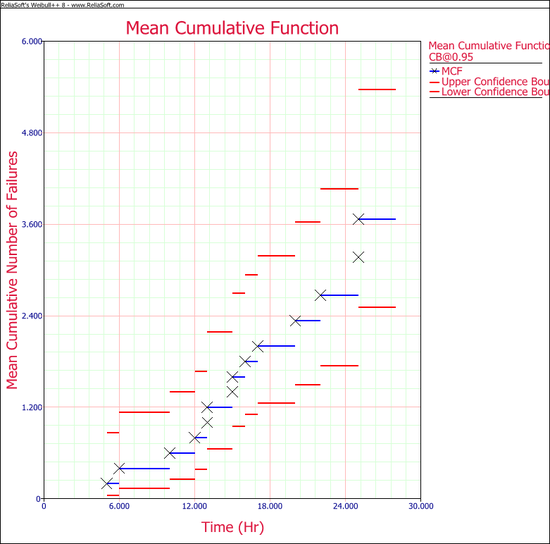
Using the equation for the MCF bounds and [math]\displaystyle{ {{K}_{5}} = 1.644\,\! }[/math] for a 95% confidence level, the confidence bounds can be obtained as follows:

[math]\displaystyle{ \begin{matrix} ID & Months & State & MC{{F}_{i}} & Va{{r}_{i}} & MC{{F}_{{{L}_{i}}}} & MC{{F}_{{{U}_{i}}}} \\ \text{1} & \text{5} & \text{F} & \text{0}\text{.20} & \text{0}\text{.032} & 0.0459 & 0.8709 \\ \text{2} & \text{6} & \text{F} & \text{0}\text{.40} & \text{0}\text{.064} & 0.1413 & 1.1320 \\ \text{1} & \text{10} & \text{F} & \text{0}\text{.60} & \text{0}\text{.096} & 0.2566 & 1.4029 \\ \text{3} & \text{12} & \text{F} & \text{0}\text{.80} & \text{0}\text{.128} & 0.3834 & 1.6694 \\ \text{2} & \text{13} & \text{F} & \text{1}\text{.00} & \text{0}\text{.160} & 0.5179 & 1.9308 \\ \text{4} & \text{13} & \text{F} & \text{1}\text{.20} & \text{0}\text{.192} & 0.6582 & 2.1879 \\ \text{1} & \text{15} & \text{F} & \text{1}\text{.40} & \text{0}\text{.224} & 0.8028 & 2.4413 \\ \text{4} & \text{15} & \text{F} & \text{1}\text{.60} & \text{0}\text{.256} & 0.9511 & 2.6916 \\ \text{5} & \text{16} & \text{F} & \text{1}\text{.80} & \text{0}\text{.288} & 1.1023 & 2.9393 \\ \text{2} & \text{17} & \text{F} & \text{2}\text{.00} & \text{0}\text{.320} & 1.2560 & 3.1848 \\ \text{1} & \text{17} & \text{S} & {} & {} & {} & {} \\ \text{2} & \text{19} & \text{S} & {} & {} & {} & {} \\ \text{3} & \text{20} & \text{F} & \text{2}\text{.33} & \text{0}\text{.394} & 1.4990 & 3.6321 \\ \text{5} & \text{22} & \text{F} & \text{2}\text{.66} & \text{0}\text{.468} & 1.7486 & 4.0668 \\ \text{4} & \text{24} & \text{S} & {} & {} & {} & {} \\ \text{3} & \text{25} & \text{F} & \text{3}\text{.16} & \text{0}\text{.593} & 2.1226 & 4.7243 \\ \text{5} & \text{25} & \text{F} & \text{3}\text{.66} & \text{0}\text{.718} & 2.5071 & 5.3626 \\ \text{3} & \text{26} & \text{S} & {} & {} & {} & {} \\ \text{5} & \text{28} & \text{S} & {} & {} & {} & {} \\ \end{matrix}\,\! }[/math]

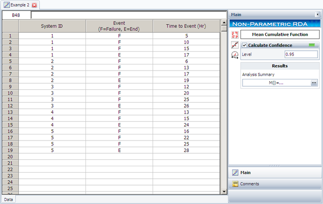
The analysis presented in this example can be performed automatically in Weibull++'s non-parametric RDA folio, as shown next.

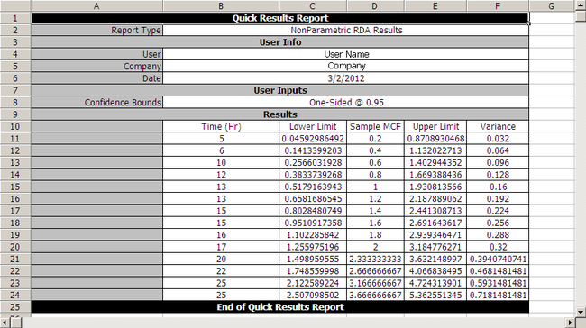
Note: In the folio above, the [math]\displaystyle{ F\,\! }[/math] refers to failures and [math]\displaystyle{ E\,\! }[/math] refers to suspensions (or censoring ages). The results, with calculated MCF values and upper and lower 95% confidence limits, are shown next along with the graphical plot.