Appendix A: Brief Statistical Background: Difference between revisions
| Line 343: | Line 343: | ||
===Single Parameter Case=== | ===Single Parameter Case=== | ||
For simplicity, consider a one parameter distribution represented by a general function <math>G,</math> which is a function of one parameter estimator, say <math>G(\widehat{\theta }).</math> Then, in general, the expected value of <math>G\left( \widehat{\theta } \right)</math> can be found by: | For simplicity, consider a one parameter distribution represented by a general function <math>G,</math> which is a function of one parameter estimator, say <math>G(\widehat{\theta }).</math> Then, in general, the expected value of <math>G\left( \widehat{\theta } \right)</math> can be found by: | ||
<br> | <br> | ||
::<math>E\left( G\left( \widehat{\theta } \right) \right)=G(\theta )+O\left( \frac{1}{n} \right)</math> | ::<math>E\left( G\left( \widehat{\theta } \right) \right)=G(\theta )+O\left( \frac{1}{n} \right)</math> | ||
where <math>G(\theta )</math> is some function of <math>\theta </math> , such as the reliability function, and <math>\theta </math> is the population moment, or parameter such that <math>E\left( \widehat{\theta } \right)=\theta </math> as | |||
where <math>G(\theta )</math> is some function of <math>\theta </math> , such as the reliability function, and <math>\theta </math> is the population moment, or parameter such that <math>E\left( \widehat{\theta } \right)=\theta </math> as <math>n\to \infty </math>. The term <math>O\left( \tfrac{1}{n} \right)</math> is a function of <math>n</math> , the sample size, and tends to zero, as fast as <math>\frac{1}{n}</math> as <math>n\to \infty .</math> For example, in the case of <math>\widehat{\theta }=\overline{x}</math> and <math>G(x)={{x}^{2}}</math> , then <math>E(G(\overline{x}))={{\mu }^{2}}+O\left( \tfrac{1}{n} \right)</math> where <math>O\left( \tfrac{1}{n} \right)=\tfrac{{{\sigma }^{2}}}{n},</math> thus as <math>n\to \infty </math> , <math>E(G(\overline{x}))={{\mu }^{2}}</math> ( <math>\mu </math> and <math>\sigma </math> are the mean and standard deviation, respectively). Using the same one parameter distribution, the variance of the function <math>G\left( \widehat{\theta } \right)</math> can then be estimated by: | |||
::<math>Var\left( G\left( \widehat{\theta } \right) \right)=\left( \frac{\partial G}{\partial \widehat{\beta }} \right)_{\widehat{\theta }=\theta }^{2}Var\left( \widehat{\theta } \right)+O\left( \frac{1}{{{n}^{\tfrac{3}{2}}}} \right)</math> | ::<math>Var\left( G\left( \widehat{\theta } \right) \right)=\left( \frac{\partial G}{\partial \widehat{\beta }} \right)_{\widehat{\theta }=\theta }^{2}Var\left( \widehat{\theta } \right)+O\left( \frac{1}{{{n}^{\tfrac{3}{2}}}} \right)</math> | ||
<br> | <br> | ||
Revision as of 18:18, 23 February 2012
Reference Appendix A: Brief Statistical Background
In this appendix we attempt to provide a brief elementary introduction to the most common and fundamental statistical equations and definitions used in reliability engineering and life data analysis. The equations and concepts presented in this appendix are used extensively throughout this reference.
Basic Statistical Definitions
Random Variables
In general, most problems in reliability engineering deal with quantitative measures, such as the time-to-failure of a product, or whether the product fails or does not fail. In judging a product to be defective or non-defective, only two outcomes are possible. We can use a random variable to denote these possible outcomes (i.e. defective or non-defective). In this case, [math]\displaystyle{ X }[/math] is a random variable that can take on only these values.
In the case of times-to-failure, our random variable [math]\displaystyle{ X }[/math] can take on the time-to-failure of the product and can be in a range from [math]\displaystyle{ 0 }[/math] to infinity (since we do not know the exact time a priori).
In the first case in which the random variable can take on discrete values (let's say [math]\displaystyle{ defective=0 }[/math] and [math]\displaystyle{ non-defective=1 }[/math] ), the variable is said to be a [math]\displaystyle{ discrete }[/math] [math]\displaystyle{ random }[/math] [math]\displaystyle{ variable. }[/math] In the second case, our product can be found failed at any time after time 0 (i.e. at 12 hr or at 100 hr and so forth), thus [math]\displaystyle{ X }[/math] can take on any value in this range. In this case, our random variable [math]\displaystyle{ X }[/math] is said to be a [math]\displaystyle{ continous }[/math] [math]\displaystyle{ random }[/math] [math]\displaystyle{ variable. }[/math] In this reference, we will deal almost exclusively with continuous random variables.
The Probability Density and Cumulative Density Functions
Designations
From probability and statistics, given a continuous random variable [math]\displaystyle{ X, }[/math] we denote:
• The probability density (distribution) function, [math]\displaystyle{ pdf }[/math] , as [math]\displaystyle{ f(x). }[/math]
• The cumulative density function, [math]\displaystyle{ cdf }[/math] , as [math]\displaystyle{ F(x). }[/math]
The [math]\displaystyle{ pdf }[/math] and [math]\displaystyle{ cdf }[/math] give a complete description of the probability distribution of a random variable.
Definitions
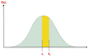
If [math]\displaystyle{ X }[/math] is a continuous random variable, then the [math]\displaystyle{ probability\ density\ function }[/math], [math]\displaystyle{ pdf }[/math] , of [math]\displaystyle{ X }[/math] is a function [math]\displaystyle{ f(x) }[/math] such that for two numbers, [math]\displaystyle{ a }[/math] and [math]\displaystyle{ b }[/math] with [math]\displaystyle{ a\le b }[/math] :
- [math]\displaystyle{ P(a\le X\le b)=\int_{a}^{b}f(x)dx }[/math]
That is, the probability that [math]\displaystyle{ X }[/math] takes on a value in the interval [math]\displaystyle{ [a,b] }[/math] is the area under the density function from [math]\displaystyle{ a }[/math] to [math]\displaystyle{ b }[/math] .
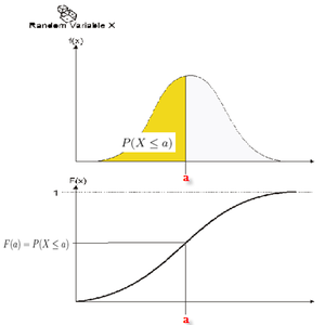
The [math]\displaystyle{ cumulative\ distribution\ function }[/math] , [math]\displaystyle{ cdf }[/math] , is a function [math]\displaystyle{ F(x), }[/math] of a random variable [math]\displaystyle{ X }[/math] , and is defined for a number [math]\displaystyle{ x }[/math] by:
- [math]\displaystyle{ F(x)=P(X\le x)=\int_{0}^{x}f(s)ds }[/math]
That is, for a number [math]\displaystyle{ x }[/math] , [math]\displaystyle{ F(x) }[/math] is the probability that the observed value of [math]\displaystyle{ X }[/math] will be at most [math]\displaystyle{ x }[/math] .
Note that depending on the function denoted by [math]\displaystyle{ f(x) }[/math] , or more specifically the distribution denoted by [math]\displaystyle{ f(x), }[/math] the limits will vary depending on the region over which the distribution is defined. For example, for all the life distributions considered in this reference, this range would be [math]\displaystyle{ [0,+\infty ]. }[/math]
Graphical representation of the [math]\displaystyle{ pdf }[/math] and [math]\displaystyle{ cdf }[/math]
Mathematical Relationship Between the [math]\displaystyle{ pdf }[/math] and [math]\displaystyle{ cdf }[/math]
The mathematical relationship between the [math]\displaystyle{ pdf }[/math] and [math]\displaystyle{ cdf }[/math] is given by:
- [math]\displaystyle{ F(x)=\int_{0}^{x}f(s)ds }[/math]
where [math]\displaystyle{ s }[/math] is a dummy integration variable.
Conversely:
- [math]\displaystyle{ f(x)=-\frac{d(F(x))}{dx} }[/math]
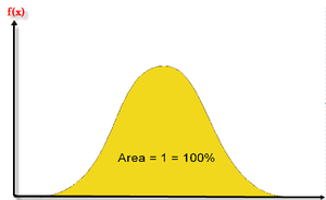
In plain English, the [math]\displaystyle{ cdf }[/math] is the area under the probability density function, up to a value of [math]\displaystyle{ x }[/math] , if so chosen. The total area under the [math]\displaystyle{ pdf }[/math] is always equal to 1, or mathematically:
- [math]\displaystyle{ \int_{0}^{\infty }f(x)dx=1 }[/math]
An example of a probability density function is the well known normal distribution, for which the [math]\displaystyle{ pdf }[/math] is given by:
- [math]\displaystyle{ f(t)=\frac{1}{\sigma \sqrt{2\pi }}{{e}^{-\tfrac{1}{2}{{\left( \tfrac{t-\mu }{\sigma } \right)}^{2}}}} }[/math]
where [math]\displaystyle{ \mu }[/math] is the mean and [math]\displaystyle{ \sigma }[/math] is the standard deviation. The normal distribution is a two parameter distribution, i.e. with two parameters [math]\displaystyle{ \mu }[/math] and [math]\displaystyle{ \sigma }[/math] .
Another is the lognormal distribution, whose [math]\displaystyle{ pdf }[/math] is given by:
- [math]\displaystyle{ f(t)=\frac{1}{t\cdot {{\sigma }^{\prime }}\sqrt{2\pi }}{{e}^{-\tfrac{1}{2}{{\left( \tfrac{{{t}^{\prime }}-{{\mu }^{\prime }}}{{{\sigma }^{\prime }}} \right)}^{2}}}} }[/math]
where [math]\displaystyle{ {\mu }' }[/math] is the mean of the natural logarithms of the times-to-failure, and [math]\displaystyle{ {\sigma }' }[/math] is the standard deviation of the natural logarithms of the times-to-failure. Again, this is a two parameter distribution.
The Reliability Function
The reliability function can be derived using the previous definition of the cumulative density function. Note that the probability of an event occurring by time [math]\displaystyle{ t }[/math] (based on a continuous distribution given by [math]\displaystyle{ f(x), }[/math] or henceforth [math]\displaystyle{ f(t) }[/math] since our random variable of interest in life data analysis is time, or [math]\displaystyle{ t }[/math] ), is given by:
- [math]\displaystyle{ F(t)=\int_{0}^{t}f(s)ds }[/math]
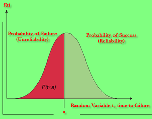
One could equate this event to the probability of a unit failing by time [math]\displaystyle{ t }[/math] .
From this fact, the most commonly used function in reliability engineering, the reliability function, can then be obtained. The reliability function enables the determination of the probability of success of a unit, in undertaking a mission of a prescribed duration.
To show this mathematically, we first define the unreliability function, [math]\displaystyle{ Q(t) }[/math] , which is the probability of failure, or the probability that our time-to-failure is in the region of [math]\displaystyle{ 0 }[/math] and [math]\displaystyle{ t }[/math] . Therefore:
- [math]\displaystyle{ F(t)=Q(t)=\int_{0}^{t}f(s)ds }[/math]
Reliability and unreliability are success and failure probabilities, are the only two events being considered, and are mutually exclusive; hence, the sum of these probabilities is equal to unity. So then:
- [math]\displaystyle{ \begin{align} Q(t)+R(t)=\ & 1 \\ R(t)=\ & 1-Q(t) \\ R(t)=\ & 1-\int_{0}^{t}f(s)ds \\ R(t)=\ & \int_{t}^{\infty }f(s)ds \end{align} }[/math]
Conversely:
- [math]\displaystyle{ f(t)=\frac{d(R(t))}{dt} }[/math]
The Failure Rate Function
The failure rate function enables the determination of the number of failures occurring per unit time. Omitting the derivation, see [18; Ch. 4], the failure rate is mathematically given as:
- [math]\displaystyle{ \lambda (t)=\frac{f(t)}{R(t)} }[/math]
Failure rate is denoted as failures per unit time.
The Mean Life Function
The mean life function, which provides a measure of the average time of operation to failure is given by:
- [math]\displaystyle{ \overline{T}=m=\int_{0}^{\infty }t\cdot f(t)dt }[/math]
This is the expected or average time-to-failure and is denoted as the [math]\displaystyle{ MTTF }[/math] (Mean Time-to-Failure) and synonymously called [math]\displaystyle{ MTBF }[/math] (Mean Time Before Failure) by many authors.
Median Life
Median life, [math]\displaystyle{ \breve{T} }[/math],
is the value of the random variable that has exactly one-half of the area under the [math]\displaystyle{ pdf }[/math] to its left and one-half to its right. The median is obtained from:
- [math]\displaystyle{ \int_{0}^{{\breve{T}}}f(t)dt=0.5 }[/math]
(For individual data, e.g. 12, 20, 21, the median is the midpoint value, or 20 in this case.)
Mode
The modal (or mode) life, [math]\displaystyle{ \tilde{T} }[/math],
is the maximum value of [math]\displaystyle{ T }[/math] that satisfies:
- [math]\displaystyle{ \frac{d\left[ f(t) \right]}{dt}=0 }[/math]
For a continuous distribution, the mode is that value of the variate which corresponds to the maximum probability density (the value at which the [math]\displaystyle{ pdf }[/math] has its maximum value).
Distributions
A statistical distribution is fully described by its [math]\displaystyle{ pdf }[/math] (probability density function). In the previous sections, we used the definition of the [math]\displaystyle{ pdf }[/math] to show how all other functions most commonly used in reliability engineering and life data analysis can be derived. The reliability function, failure rate function, mean time function, and median life function can be determined directly from the [math]\displaystyle{ pdf }[/math] definition, or [math]\displaystyle{ f(t) }[/math] . Different distributions exist, such as the normal, exponential, etc., and each has a predefined [math]\displaystyle{ f(t) }[/math] which can be found in most references. These distributions were formulated by statisticians, mathematicians and/or engineers to mathematically model or represent certain behavior. For example, the Weibull distribution was formulated by Waloddi Weibull and thus it bears his name. Some distributions tend to better represent life data and are most commonly called lifetime distributions.
The exponential distribution is a very commonly used distribution in reliability engineering. Due to its simplicity, it has been widely employed even in cases to which it does not apply. The [math]\displaystyle{ pdf }[/math] of the exponential distribution is mathematically defined as:
- [math]\displaystyle{ f(t)=\lambda {{e}^{-\lambda t}} }[/math]
In this definition, note that [math]\displaystyle{ t }[/math] is our random variable, which represents time, and the Greek letter [math]\displaystyle{ \lambda }[/math] (lambda) represents what is commonly referred to as the parameter of the distribution. For any distribution, the parameter or parameters of the distribution are estimated (obtained) from the data. For example, in the case of the most well known distribution, namely the normal distribution:
- [math]\displaystyle{ f(t)=\frac{1}{\sigma \sqrt{2\pi }}{{e}^{-\tfrac{1}{2}{{\left( \tfrac{t-\mu }{\sigma } \right)}^{2}}}} }[/math]
where the mean, [math]\displaystyle{ \mu , }[/math] and the standard deviation, [math]\displaystyle{ \sigma , }[/math] are its parameters. Both of these parameters are estimated from the data, i.e. the mean and standard deviation of the data. Once these parameters are estimated, our function [math]\displaystyle{ f(t) }[/math] is fully defined and we can obtain any value for [math]\displaystyle{ f(t) }[/math] given any value of [math]\displaystyle{ t }[/math] .
Given the mathematical representation of a distribution, we can also derive all of the functions needed for life data analysis, which again will only depend on the value of [math]\displaystyle{ t }[/math] after the value of the distribution parameter or parameters are estimated from data.
For example, we know that the exponential distribution [math]\displaystyle{ pdf }[/math] is given by:
- [math]\displaystyle{ f(t)=\lambda {{e}^{-\lambda t}} }[/math]
Thus the reliability function can be derived:
- [math]\displaystyle{ \begin{align} R(t)=\ & 1-\int_{0}^{t}\lambda {{e}^{-\lambda T}}dT = 1-\left[ 1-{{e}^{-\lambda (t)}} \right] = {{e}^{-\lambda (t)}} \end{align} }[/math]
The failure rate function is given by:
- [math]\displaystyle{ \begin{align} \lambda (t)=\ & \frac{f(t)}{R(t)} = \frac{\lambda {{e}^{-\lambda (t)}}}{{{e}^{-\lambda (t)}}} = \lambda \end{align} }[/math]
The mean time to/before failure (MTTF / MTBF) is given by:
- [math]\displaystyle{ \begin{align} & \overline{T}= \underset{0}{\overset{\infty }{\mathop \int }}\,t\cdot f(t)dt = \underset{0}{\overset{\infty }{\mathop \int }}\,t\cdot \lambda \cdot {{e}^{-\lambda t}}dt = \frac{1}{\lambda } \end{align} }[/math]
Exactly the same methodology can be applied to any distribution given its [math]\displaystyle{ pdf, }[/math] with various degrees of difficulty depending on the complexity of [math]\displaystyle{ f(t) }[/math] .
Most Commonly Used Distributions
There are many different lifetime distributions that can be used. ReliaSoft [31] presents a thorough overview of lifetime distributions. Leemis [22] and others also present good overviews of many of these distributions. The three distributions used in ALTA, the 1-parameter exponential, 2-parameter Weibull, and the lognormal, are presented in greater detail here.
Confidence Intervals (or Bounds)
One of the most confusing concepts to an engineer new to the field is the concept of putting a probability on a probability. In life data analysis, this concept is referred to as confidence intervals or confidence bounds. In this section, we will try to briefly present the concept, in less than statistical terms, but based on solid common sense.
The Black and White Marbles
To illustrate, imagine a situation in which there are millions of black and white marbles in a rather large swimming pool, and our job is to estimate the percentage of black marbles. One way to do this (other than counting all the marbles!) is to estimate the percentage of black marbles by taking a sample and then counting the number of black marbles in the sample.
Taking a Small Sample of Marbles
First, let's pick out a small sample of marbles and count the black ones. Say you picked out 10 marbles and counted 4 black marbles. Based on this, your estimate would be that 40% of the marbles are black.
If you put the 10 marbles back into the pool and repeated this example, you might get 5 black marbles, changing your estimate to 50% black marbles.
Which of the two estimates is correct? Both estimates are correct! As you repeat this experiment over and over again, you might find out that this estimate is usually between [math]\displaystyle{ {{X}_{1}}% }[/math] and [math]\displaystyle{ {{X}_{2}}% }[/math] , or maybe 90% of the time this estimate is between [math]\displaystyle{ {{X}_{1}}% }[/math] and [math]\displaystyle{ {{X}_{2}}%. }[/math]
Taking a Larger Sample of Marbles
If we now repeat the experiment and pick out 1,000 marbles, we might get results such as 545, 570, 530, etc. for the number of black marbles in each trial. Note that the range in this case will be much narrower than before. For example, let's say that 90% of the time, the number of black marbles will be from [math]\displaystyle{ {{Y}_{1}}% }[/math] to [math]\displaystyle{ {{Y}_{2}}% }[/math] , where [math]\displaystyle{ {{X}_{1}}%\lt {{Y}_{1}}% }[/math] and [math]\displaystyle{ {{X}_{2}}%\gt {{Y}_{2}}% }[/math] , thus giving us a narrower interval. For confidence intervals, the larger the sample size, the narrower the confidence intervals.
Back to Reliability
Returning to the subject at hand, our task is to determine the probability of failure or reliability of all of our units. However, until all units fail, we will never know the exact value. Our task is to estimate the reliability based on a sample, much like estimating the number of black marbles in the pool. If we perform 10 different reliability tests for our units, and estimate the parameters using ALTA, we will obtain slightly different parameters for the distribution each time, and thus slightly different reliability results. However, when employing confidence bounds, we obtain a range in which these values are more likely to occur [math]\displaystyle{ X }[/math] percent of the time. Remember that each parameter is an estimate of the true parameter, a true parameter that is unknown to us.
One-Sided and Two-Sided Confidence Bounds
Confidence bounds (or intervals) are generally described as one-sided or two-sided.
Two-Sided Bounds
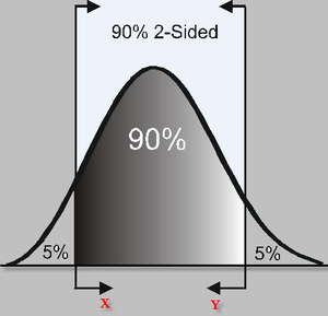
When we use two-sided confidence bounds (or intervals), we are looking at where most of the population is likely to lie. For example, when using 90% two-sided confidence bounds, we are saying that 90% lies between [math]\displaystyle{ X }[/math] and [math]\displaystyle{ Y }[/math] , with 5% less than [math]\displaystyle{ X }[/math] and 5% greater than [math]\displaystyle{ Y }[/math] .
One-Sided Bounds
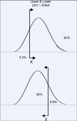
When using one-sided intervals, we are looking at the percentage of units that are greater or less (upper and lower) than a certain point [math]\displaystyle{ X }[/math] .
For example, 95% one-sided confidence bounds would indicate that 95% of the population is greater than [math]\displaystyle{ X }[/math] (if 95% is a lower confidence bound), or that 95% is less than [math]\displaystyle{ X }[/math] (if 95% is an upper confidence bound).
In ALTA, we use upper to mean the higher limit and lower to mean the lower limit, regardless of their position, but based on the value of the results. So for example, when returning the confidence bounds on the reliability, we would term the lower value of reliability as the lower limit and the higher value of reliability as the higher limit. When returning the confidence bounds on probability of failure, we will again term the lower numeric value for the probability of failure as the lower limit and the higher value as the higher limit.
Confidence Limits Determination
This section presents an overview of the theory on obtaining approximate confidence bounds on suspended (multiply censored) data. The methodology used is the so-called Fisher Matrix Bounds, described in Nelson [27] and Lloyd and Lipow [24].
Suggested References
This section presents a brief introduction into how the confidence intervals are calculated by ALTA. By no means do we intend to cover the full theory behind this methodology. More complete details on confidence intervals can be found in the following books:
• Nelson, Wayne, Applied Life Data Analysis, 1982, John Wiley & Sons, New York, New York.
• Nelson, Wayne, Accelerated Testing: Statistical Models, Test Plans, and Data Analyses, 1990, John Wiley & Sons, New York, New York.
• David K. Lloyd and Myron Lipow, Reliability: Management, Methods, and Mathematics, 1962, Prentice Hall, Englewood Cliffs, New Jersey.
• H. Cramer, Mathematical Methods of Statistics, 1946, Princeton University Press, Princeton, New Jersey.
Approximate Estimates of the Mean and Variance of a Function
Single Parameter Case
For simplicity, consider a one parameter distribution represented by a general function [math]\displaystyle{ G, }[/math] which is a function of one parameter estimator, say [math]\displaystyle{ G(\widehat{\theta }). }[/math] Then, in general, the expected value of [math]\displaystyle{ G\left( \widehat{\theta } \right) }[/math] can be found by:
- [math]\displaystyle{ E\left( G\left( \widehat{\theta } \right) \right)=G(\theta )+O\left( \frac{1}{n} \right) }[/math]
where [math]\displaystyle{ G(\theta ) }[/math] is some function of [math]\displaystyle{ \theta }[/math] , such as the reliability function, and [math]\displaystyle{ \theta }[/math] is the population moment, or parameter such that [math]\displaystyle{ E\left( \widehat{\theta } \right)=\theta }[/math] as [math]\displaystyle{ n\to \infty }[/math]. The term [math]\displaystyle{ O\left( \tfrac{1}{n} \right) }[/math] is a function of [math]\displaystyle{ n }[/math] , the sample size, and tends to zero, as fast as [math]\displaystyle{ \frac{1}{n} }[/math] as [math]\displaystyle{ n\to \infty . }[/math] For example, in the case of [math]\displaystyle{ \widehat{\theta }=\overline{x} }[/math] and [math]\displaystyle{ G(x)={{x}^{2}} }[/math] , then [math]\displaystyle{ E(G(\overline{x}))={{\mu }^{2}}+O\left( \tfrac{1}{n} \right) }[/math] where [math]\displaystyle{ O\left( \tfrac{1}{n} \right)=\tfrac{{{\sigma }^{2}}}{n}, }[/math] thus as [math]\displaystyle{ n\to \infty }[/math] , [math]\displaystyle{ E(G(\overline{x}))={{\mu }^{2}} }[/math] ( [math]\displaystyle{ \mu }[/math] and [math]\displaystyle{ \sigma }[/math] are the mean and standard deviation, respectively). Using the same one parameter distribution, the variance of the function [math]\displaystyle{ G\left( \widehat{\theta } \right) }[/math] can then be estimated by:
- [math]\displaystyle{ Var\left( G\left( \widehat{\theta } \right) \right)=\left( \frac{\partial G}{\partial \widehat{\beta }} \right)_{\widehat{\theta }=\theta }^{2}Var\left( \widehat{\theta } \right)+O\left( \frac{1}{{{n}^{\tfrac{3}{2}}}} \right) }[/math]
Two Parameter Case
Repeating the previous method for the case of a two parameter distribution, it is generally true that for a function [math]\displaystyle{ G }[/math] , which is a function of two parameter estimators, say [math]\displaystyle{ G\left( {{\widehat{\theta }}_{1}},{{\widehat{\theta }}_{2}} \right) }[/math] , that:
- [math]\displaystyle{ E\left( G\left( {{\widehat{\theta }}_{1}},{{\widehat{\theta }}_{2}} \right) \right)=G\left( {{\theta }_{1}},{{\theta }_{2}} \right)+O\left( \frac{1}{n} \right) }[/math]
- and:
- [math]\displaystyle{ \begin{align} & Var\left( G\left( {{\widehat{\theta }}_{1}},{{\widehat{\theta }}_{2}} \right) \right)= & \left( \frac{\partial G}{\partial {{\widehat{\theta }}_{1}}} \right)_{{{\widehat{\theta }}_{1}}={{\theta }_{1}}}^{2}Var\left( {{\widehat{\theta }}_{1}} \right)+\left( \frac{\partial G}{\partial {{\widehat{\theta }}_{2}}} \right)_{{{\widehat{\theta }}_{2}}={{\theta }_{1}}}^{2}Var\left( {{\widehat{\theta }}_{2}} \right) \\ & & +2{{\left( \frac{\partial G}{\partial {{\widehat{\theta }}_{1}}} \right)}_{{{\widehat{\theta }}_{1}}={{\theta }_{1}}}}{{\left( \frac{\partial G}{\partial {{\widehat{\theta }}_{2}}} \right)}_{{{\widehat{\theta }}_{2}}={{\theta }_{1}}}}Cov\left( {{\widehat{\theta }}_{1}},{{\widehat{\theta }}_{2}} \right)+O\left( \frac{1}{{{n}^{\tfrac{3}{2}}}} \right) \end{align} }[/math]
Note that the derivatives of Eqn. (var) are evaluated at [math]\displaystyle{ {{\widehat{\theta }}_{1}}={{\theta }_{1}} }[/math] and [math]\displaystyle{ {{\widehat{\theta }}_{2}}={{\theta }_{1}}, }[/math] where E [math]\displaystyle{ \left( {{\widehat{\theta }}_{1}} \right)\simeq {{\theta }_{1}} }[/math] and E [math]\displaystyle{ \left( {{\widehat{\theta }}_{2}} \right)\simeq {{\theta }_{2}}. }[/math]
Variance and Covariance Determination of the Parameters
The determination of the variance and covariance of the parameters is accomplished via the use of the Fisher information matrix. For a two parameter distribution, and using maximum likelihood estimates, the log likelihood function for censored data (without the constant coefficient) is given by:
- [math]\displaystyle{ \begin{align} & \ln [L]= & \Lambda =\underset{i=1}{\overset{R}{\mathop \sum }}\,\ln [f({{T}_{i}};{{\theta }_{1}},{{\theta }_{2}})] \\ & & \text{ }+\underset{j=1}{\overset{M}{\mathop \sum }}\,\ln [1-F({{S}_{j}};{{\theta }_{1}},{{\theta }_{2}})] \\ & & \text{ }+\underset{k=1}{\overset{P}{\mathop \sum }}\,\ln F({{I}_{i}};{{\theta }_{1}},{{\theta }_{2}})-F({{I}_{i-1}};{{\theta }_{1}},{{\theta }_{2}})\} \end{align} }[/math]
Then the Fisher information matrix is given by:
- [math]\displaystyle{ {{F}_{0}}=\left[ \begin{matrix} {{E}_{0}}{{\left[ -\tfrac{{{\partial }^{2}}\Lambda }{\partial \theta _{1}^{2}} \right]}_{0}} & {} & {{E}_{0}}{{\left[ -\tfrac{{{\partial }^{2}}\Lambda }{\partial {{\theta }_{1}}\partial {{\theta }_{2}}} \right]}_{0}} \\ {} & {} & {} \\ {{E}_{0}}{{\left[ -\tfrac{{{\partial }^{2}}\Lambda }{\partial {{\theta }_{2}}\partial {{\theta }_{1}}} \right]}_{0}} & {} & {{E}_{0}}{{\left[ -\tfrac{{{\partial }^{2}}\Lambda }{\partial \theta _{2}^{2}} \right]}_{0}} \\ \end{matrix} \right] }[/math]
- where
- [math]\displaystyle{ {{\theta }_{1}}={{\theta }_{{{1}_{0}}}}, }[/math] and [math]\displaystyle{ {{\theta }_{2}}={{\theta }_{{{2}_{0}}}}. }[/math]
So for a sample of [math]\displaystyle{ N }[/math] units where [math]\displaystyle{ R }[/math] units have failed, [math]\displaystyle{ S }[/math] have been suspended, and [math]\displaystyle{ P }[/math] have failed within a time interval, and [math]\displaystyle{ N=R+M+P, }[/math] one could obtain the sample local information matrix by:
- [math]\displaystyle{ F=\left[ \begin{matrix} -\tfrac{{{\partial }^{2}}\Lambda }{\partial \theta _{1}^{2}} & {} & -\tfrac{{{\partial }^{2}}\Lambda }{\partial {{\theta }_{1}}\partial {{\theta }_{2}}} \\ {} & {} & {} \\ -\tfrac{{{\partial }^{2}}\Lambda }{\partial {{\theta }_{2}}\partial {{\theta }_{1}}} & {} & -\tfrac{{{\partial }^{2}}\Lambda }{\partial \theta _{2}^{2}} \\ \end{matrix} \right] }[/math]
By substituting in the values of the estimated parameters, in this case [math]\displaystyle{ {{\widehat{\theta }}_{1}} }[/math] and [math]\displaystyle{ {{\widehat{\theta }}_{2}}, }[/math] and inverting the matrix, one can then obtain the local estimate of the covariance matrix or,
- [math]\displaystyle{ {{F}^{-1}}={{\left[ \begin{matrix} -\tfrac{{{\partial }^{2}}\Lambda }{\partial \theta _{1}^{2}} & {} & -\tfrac{{{\partial }^{2}}\Lambda }{\partial {{\theta }_{1}}\partial {{\theta }_{2}}} \\ {} & {} & {} \\ -\tfrac{{{\partial }^{2}}\Lambda }{\partial {{\theta }_{2}}\partial {{\theta }_{1}}} & {} & -\tfrac{{{\partial }^{2}}\Lambda }{\partial \theta _{2}^{2}} \\ \end{matrix} \right]}^{-1}}=\left[ \begin{matrix} Var\left( {{\widehat{\theta }}_{1}} \right) & {} & Cov\left( {{\widehat{\theta }}_{1}},{{\widehat{\theta }}_{2}} \right) \\ {} & {} & {} \\ Cov\left( {{\widehat{\theta }}_{1}},{{\widehat{\theta }}_{2}} \right) & {} & Var\left( {{\widehat{\theta }}_{2}} \right) \\ \end{matrix} \right] }[/math]
Then the variance of a function ( [math]\displaystyle{ Var(G) }[/math] ) can be estimated using Eqn. (var). Values for the variance and covariance of the parameters are obtained from Eqn. (Fisher2). Once they are obtained, the approximate confidence bounds on the function are given as:
- [math]\displaystyle{ C{{B}_{R}}=E(G)\pm {{z}_{\alpha }}\sqrt{Var(G)} }[/math]
Approximate Confidence Intervals on the Parameters
In general, MLE estimates of the parameters are asymptotically normal, thus if [math]\displaystyle{ \widehat{\theta } }[/math] is the MLE estimator for [math]\displaystyle{ \theta }[/math] , in the case of a single parameter distribution, estimated from a sample of [math]\displaystyle{ n }[/math] units, and if:
- [math]\displaystyle{ z\equiv \frac{\widehat{\theta }-\theta }{\sqrt{Var\left( \widehat{\theta } \right)}} }[/math]
then:
- [math]\displaystyle{ P\left( z\le x \right)\to \Phi \left( z \right)=\frac{1}{\sqrt{2\pi }}\mathop{}_{-\infty }^{x}{{e}^{-\tfrac{{{t}^{2}}}{2}}}dt }[/math]
for large [math]\displaystyle{ n }[/math] . If one now wishes to place confidence bounds on [math]\displaystyle{ \theta , }[/math] at some confidence level [math]\displaystyle{ \delta }[/math] , bounded by the two end points [math]\displaystyle{ {{C}_{1}} }[/math] and [math]\displaystyle{ {{C}_{2}} }[/math] , and where:
- [math]\displaystyle{ P\left( {{C}_{1}}\lt \theta \lt {{C}_{2}} \right)=\delta }[/math]
then from Eqn. (e729):
- [math]\displaystyle{ P\left( -{{K}_{\tfrac{1-\delta }{2}}}\lt \frac{\widehat{\theta }-\theta }{\sqrt{Var\left( \widehat{\theta } \right)}}\lt {{K}_{\tfrac{1-\delta }{2}}} \right)\simeq \delta }[/math]
where [math]\displaystyle{ {{K}_{\alpha }} }[/math] is defined by:
- [math]\displaystyle{ \alpha =\frac{1}{\sqrt{2\pi }}\mathop{}_{{{K}_{\alpha }}}^{\infty }{{e}^{-\tfrac{{{t}^{2}}}{2}}}dt=1-\Phi \left( {{K}_{\alpha }} \right) }[/math]
Now by simplifying Eqn. (e731), one can obtain the approximate confidence bounds on the parameter [math]\displaystyle{ \theta , }[/math] at a confidence level [math]\displaystyle{ \delta }[/math] or:
- [math]\displaystyle{ \left( \widehat{\theta }-{{K}_{\tfrac{1-\delta }{2}}}\cdot \sqrt{Var\left( \widehat{\theta } \right)}\lt \theta \lt \widehat{\theta }+{{K}_{\tfrac{1-\delta }{2}}}\cdot \sqrt{Var\left( \widehat{\theta } \right)} \right) }[/math]
If [math]\displaystyle{ \widehat{\theta } }[/math] must be positive, then [math]\displaystyle{ \ln \widehat{\theta } }[/math] is treated as normally distributed. The two-sided approximate confidence bounds on the parameter [math]\displaystyle{ \theta }[/math] , at confidence level [math]\displaystyle{ \delta }[/math] , then become:
- [math]\displaystyle{ \begin{align} & {{\theta }_{U}}= & \widehat{\theta }\cdot {{e}^{\tfrac{{{K}_{\tfrac{1-\delta }{2}}}\sqrt{Var\left( \widehat{\theta } \right)}}{\widehat{\theta }}}}\text{ (Two-sided Upper)} \\ & {{\theta }_{L}}= & \frac{\widehat{\theta }}{{{e}^{\tfrac{{{K}_{\tfrac{1-\delta }{2}}}\sqrt{Var\left( \widehat{\theta } \right)}}{\widehat{\theta }}}}}\text{ (Two-sided Lower)} \end{align} }[/math]
The one-sided approximate confidence bounds on the parameter [math]\displaystyle{ \theta }[/math] , at confidence level [math]\displaystyle{ \delta }[/math] can be found from:
- [math]\displaystyle{ \begin{align} & {{\theta }_{U}}= & \widehat{\theta }\cdot {{e}^{\tfrac{{{K}_{1-\delta }}\sqrt{Var\left( \widehat{\theta } \right)}}{\widehat{\theta }}}}\text{ (One-sided Upper)} \\ & {{\theta }_{L}}= & \frac{\widehat{\theta }}{{{e}^{\tfrac{{{K}_{1-\delta }}\sqrt{Var\left( \widehat{\theta } \right)}}{\widehat{\theta }}}}}\text{ (One-sided Lower)} \end{align} }[/math]
The same procedure can be repeated for the case of a two or more parameter distribution. Lloyd and Lipow [24] elaborate on this procedure.
Percentile Confidence Bounds (Type 1 in ALTA)
Percentile confidence bounds are confidence bounds around time. For example, when using the 1-parameter exponential distribution, the corresponding time for a given exponential percentile (i.e., y-ordinate or unreliability, [math]\displaystyle{ Q=1-R) }[/math] is determined by solving the unreliability function for the time, [math]\displaystyle{ T }[/math] , or:
- [math]\displaystyle{ \begin{align} & T(Q)= & -\frac{1}{\widehat{\lambda }}\ln (1-Q) \\ & = & -\frac{1}{\widehat{\lambda }}\ln (R) \end{align} }[/math]
Percentile bounds (Type 1) return the confidence bounds by determining the confidence intervals around [math]\displaystyle{ \widehat{\lambda } }[/math] and substituting into Eqn. (cb). The bounds on [math]\displaystyle{ \widehat{\lambda } }[/math] were determined using Eqns. (cblmu) and (cblml), with its variance obtained from Eqn. (Fisher2).
Reliability Confidence Bounds (Type 2 in ALTA)
Type 2 bounds in ALTA are confidence bounds around reliability. For example, when using the 1-parameter exponential distribution, the reliability function is:
- [math]\displaystyle{ R(T)={{e}^{-\widehat{\lambda }\cdot T}} }[/math]
Reliability bounds (Type 2) return the confidence bounds by determining the confidence intervals around [math]\displaystyle{ \widehat{\lambda } }[/math] and substituting into Eqn. (cbr). The bounds on [math]\displaystyle{ \widehat{\lambda } }[/math] were determined using Eqns. (cblmu) and (cblml), with its variance obtained from Eqn. (Fisher2).


