Distributions Used in Accelerated Testing: Difference between revisions
No edit summary |
Chris Kahn (talk | contribs) m (moved Distributions used in Accelerated Testing to Distributions Used in Accelerated Testing: Changed capitalization in title.) |
(No difference)
| |
Revision as of 22:17, 6 March 2012
Life Distributions
In this section we will briefly present three lifetime distributions commonly used in accelerated
life test analysis, namely the 1-parameter exponential, the 2-parameter Weibull and the lognormal
distributions. Readers who are interested in a more rigorous overview or in different forms of
these and other life distributions can refer to ReliaSoft's Life Data Analysis Reference.
Template loop detected: Template:Alta exponential distribution
Parameter Estimation
The parameter of the exponential distribution can be estimated graphically on probability plotting paper or analytically using either least squares or maximum likelihood. (Parameter estimation methods are presented in detail in Appendix B.)
Let's assume six identical units are reliability tested at the same application and operation
stress levels. All of these units fail during the test after operating for the following times (in hours): 96, 257, 498, 763, 1051 and 1744.
The steps for using the probability plotting method to determine the parameters of the exponential pdf representing the data are as follows:
Rank the times-to-failure in ascending order as shown next.
Obtain their median rank plotting positions. Median rank positions are used instead of other ranking methods because median ranks are at a specific confidence level (50%).
The times-to-failure, with their corresponding median ranks, are shown next:
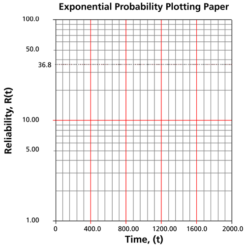
On an exponential probability paper, plot the times on the x-axis and their corresponding rank value on the y-axis. The next figure displays an example of an exponential probability paper. The paper is simply a log-linear paper.
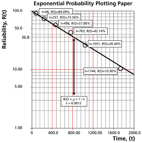
Draw the best possible straight line that goes through the [math]\displaystyle{ t=0\,\! }[/math] and [math]\displaystyle{ (t)=100%\,\! }[/math] point and through the plotted points (as shown in the plot below).
At the [math]\displaystyle{ Q(t)=63.2%\,\! }[/math] or [math]\displaystyle{ R(t)=36.8%\,\! }[/math] ordinate point, draw a straight horizontal line until this line intersects the fitted straight line. Draw a vertical line through this intersection until it crosses the abscissa. The value at the intersection of the abscissa is the estimate of the mean. For this case, [math]\displaystyle{ \widehat{\mu }=833\,\! }[/math] hours which means that [math]\displaystyle{ \lambda =\tfrac{1}{\mu }=0.0012\,\! }[/math] (This is always at 63.2% because [math]\displaystyle{ (T)=1-{{e}^{-\tfrac{\mu }{\mu }}}=1-{{e}^{-1}}=0.632=63.2%)\,\! }[/math].
Now any reliability value for any mission time [math]\displaystyle{ t\,\! }[/math] can be obtained. For example, the reliability for a mission of 15 hours, or any other time, can now be obtained either from the plot or analytically.
To obtain the value from the plot, draw a vertical line from the abscissa, at [math]\displaystyle{ t=15\,\! }[/math] hours, to the fitted line. Draw a horizontal line from this intersection to the ordinate and read [math]\displaystyle{ R(t)\,\! }[/math]. In this case, [math]\displaystyle{ R(t=15)=98.15%\,\! }[/math]. This can also be obtained analytically, from the exponential reliability function.
Template loop detected: Template:Alta weibull distribution
Template loop detected: Template:Alta ld
Parameter Estimation
The parameter of the exponential distribution can be estimated graphically on probability plotting paper or analytically using either least squares or maximum likelihood. (Parameter estimation methods are presented in detail in Appendix B.)
Let's assume six identical units are reliability tested at the same application and operation
stress levels. All of these units fail during the test after operating for the following times (in hours): 96, 257, 498, 763, 1051 and 1744.
The steps for using the probability plotting method to determine the parameters of the exponential pdf representing the data are as follows:
Rank the times-to-failure in ascending order as shown next.
Obtain their median rank plotting positions. Median rank positions are used instead of other ranking methods because median ranks are at a specific confidence level (50%).
The times-to-failure, with their corresponding median ranks, are shown next:
On an exponential probability paper, plot the times on the x-axis and their corresponding rank value on the y-axis. The next figure displays an example of an exponential probability paper. The paper is simply a log-linear paper.
Draw the best possible straight line that goes through the [math]\displaystyle{ t=0\,\! }[/math] and [math]\displaystyle{ (t)=100%\,\! }[/math] point and through the plotted points (as shown in the plot below).
At the [math]\displaystyle{ Q(t)=63.2%\,\! }[/math] or [math]\displaystyle{ R(t)=36.8%\,\! }[/math] ordinate point, draw a straight horizontal line until this line intersects the fitted straight line. Draw a vertical line through this intersection until it crosses the abscissa. The value at the intersection of the abscissa is the estimate of the mean. For this case, [math]\displaystyle{ \widehat{\mu }=833\,\! }[/math] hours which means that [math]\displaystyle{ \lambda =\tfrac{1}{\mu }=0.0012\,\! }[/math] (This is always at 63.2% because [math]\displaystyle{ (T)=1-{{e}^{-\tfrac{\mu }{\mu }}}=1-{{e}^{-1}}=0.632=63.2%)\,\! }[/math].
Now any reliability value for any mission time [math]\displaystyle{ t\,\! }[/math] can be obtained. For example, the reliability for a mission of 15 hours, or any other time, can now be obtained either from the plot or analytically.
To obtain the value from the plot, draw a vertical line from the abscissa, at [math]\displaystyle{ t=15\,\! }[/math] hours, to the fitted line. Draw a horizontal line from this intersection to the ordinate and read [math]\displaystyle{ R(t)\,\! }[/math]. In this case, [math]\displaystyle{ R(t=15)=98.15%\,\! }[/math]. This can also be obtained analytically, from the exponential reliability function.
Life Distributions
In this section we will briefly present three lifetime distributions commonly used in accelerated
life test analysis, namely the 1-parameter exponential, the 2-parameter Weibull and the lognormal
distributions. Readers who are interested in a more rigorous overview or in different forms of
these and other life distributions can refer to ReliaSoft's Life Data Analysis Reference.
Template loop detected: Template:Alta exponential distribution
Parameter Estimation
The parameter of the exponential distribution can be estimated graphically on probability plotting paper or analytically using either least squares or maximum likelihood. (Parameter estimation methods are presented in detail in Appendix B.)
Let's assume six identical units are reliability tested at the same application and operation
stress levels. All of these units fail during the test after operating for the following times (in hours): 96, 257, 498, 763, 1051 and 1744.
The steps for using the probability plotting method to determine the parameters of the exponential pdf representing the data are as follows:
Rank the times-to-failure in ascending order as shown next.
Obtain their median rank plotting positions. Median rank positions are used instead of other ranking methods because median ranks are at a specific confidence level (50%).
The times-to-failure, with their corresponding median ranks, are shown next:
On an exponential probability paper, plot the times on the x-axis and their corresponding rank value on the y-axis. The next figure displays an example of an exponential probability paper. The paper is simply a log-linear paper.
Draw the best possible straight line that goes through the [math]\displaystyle{ t=0\,\! }[/math] and [math]\displaystyle{ (t)=100%\,\! }[/math] point and through the plotted points (as shown in the plot below).
At the [math]\displaystyle{ Q(t)=63.2%\,\! }[/math] or [math]\displaystyle{ R(t)=36.8%\,\! }[/math] ordinate point, draw a straight horizontal line until this line intersects the fitted straight line. Draw a vertical line through this intersection until it crosses the abscissa. The value at the intersection of the abscissa is the estimate of the mean. For this case, [math]\displaystyle{ \widehat{\mu }=833\,\! }[/math] hours which means that [math]\displaystyle{ \lambda =\tfrac{1}{\mu }=0.0012\,\! }[/math] (This is always at 63.2% because [math]\displaystyle{ (T)=1-{{e}^{-\tfrac{\mu }{\mu }}}=1-{{e}^{-1}}=0.632=63.2%)\,\! }[/math].
Now any reliability value for any mission time [math]\displaystyle{ t\,\! }[/math] can be obtained. For example, the reliability for a mission of 15 hours, or any other time, can now be obtained either from the plot or analytically.
To obtain the value from the plot, draw a vertical line from the abscissa, at [math]\displaystyle{ t=15\,\! }[/math] hours, to the fitted line. Draw a horizontal line from this intersection to the ordinate and read [math]\displaystyle{ R(t)\,\! }[/math]. In this case, [math]\displaystyle{ R(t=15)=98.15%\,\! }[/math]. This can also be obtained analytically, from the exponential reliability function.
Template loop detected: Template:Alta weibull distribution
Template loop detected: Template:Alta ld


