Template:Example: Normal General Example (RRX Plot): Difference between revisions
No edit summary |
No edit summary |
||
| Line 14: | Line 14: | ||
<math></math> | <math></math> | ||
[[Image: | [[Image:Normal Distribution Example 8 Data.png|thumb|center|400px| ]] | ||
| Line 26: | Line 26: | ||
<math></math> | <math></math> | ||
[[Image: | [[Image:Normal Distribution Example 8 Probability Plot.png|thumb|center|400px| ]] | ||
3. From the | 3. From the '''Plot Type''' menu choose Pdf Plot. The following plot should appear on your screen. | ||
[[Image: | [[Image:Normal Distribution Example 8 pdf Plot.png|thumb|center|400px| ]] | ||
<math></math> | <math></math> | ||
Revision as of 00:03, 2 March 2012
Normal General Example (RRX Plot)
Six units are tested to failure with the following hours-to-failure data obtained: 12125, 11260, 12080, 12825, 13550 and 14670 hours. Assuming the data are normally distributed, do the following:
1. Find the parameters for the data. (Use Rank Regression on X to duplicate the results shown in this example.)
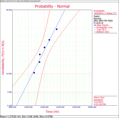
2. Obtain the probability plot for the data with 90%, two-sided Type 1 confidence bounds.
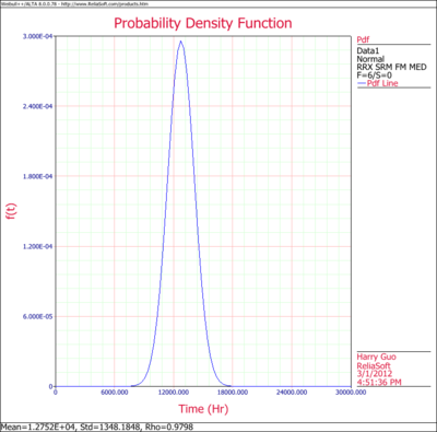
3. Obtain the [math]\displaystyle{ pdf }[/math] plot for these data.
Solutions
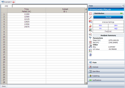
1. The next figure shows the data as entered in Weibull++, as well as the calculated parameters.
[math]\displaystyle{ }[/math]
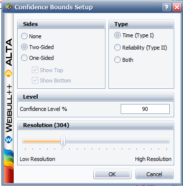
2. Obtain the probability plot as before. To plot confidence bounds, from the Plot Options menu choose Confidence Bounds and then Show Confidence Bounds. On the Type and Settings page of the Confidence Bounds window, select Two Sided Bounds, make sure Type 1 is selected, and then enter 90 in the Confidence level, % box, and click OK, as shown next.
[math]\displaystyle{ }[/math]
The following plot should appear on your screen:
[math]\displaystyle{ }[/math]
3. From the Plot Type menu choose Pdf Plot. The following plot should appear on your screen.
[math]\displaystyle{ }[/math]


