Template:Likelihood Ratio Confidence Bounds: Difference between revisions
| Line 44: | Line 44: | ||
:#<math>L(\widehat{\theta })</math> is the likelihood function calculated at the estimated vector <math>\widehat{\theta }</math> | :#<math>L(\widehat{\theta })</math> is the likelihood function calculated at the estimated vector <math>\widehat{\theta }</math> | ||
:#<math>\chi _{\alpha ;k}^{2}</math> is the chi-squared statistic with probability <math>\alpha </math> and <math>k</math> degrees of freedom, where <math>k</math> is the number of quantities jointly estimated | :#<math>\chi _{\alpha ;k}^{2}</math> is the chi-squared statistic with probability <math>\alpha </math> and <math>k</math> degrees of freedom, where <math>k</math> is the number of quantities jointly estimated | ||
If <math>\delta </math> is the confidence level, then <math>\alpha =\delta </math> for two-sided bounds and <math>\alpha =(2\delta -1)</math> for one-sided. Recall from Chapter | If <math>\delta </math> is the confidence level, then <math>\alpha =\delta </math> for two-sided bounds and <math>\alpha =(2\delta -1)</math> for one-sided. Recall from Chapter [[Basic Statistical Background]] that if <math>x</math> is a continuous random variable with <math>pdf</math>: | ||
::<math>f(x;{{\theta }_{1}},{{\theta }_{2}},...,{{\theta }_{k}})</math>, | ::<math>f(x;{{\theta }_{1}},{{\theta }_{2}},...,{{\theta }_{k}})</math>, | ||
| Line 61: | Line 61: | ||
'''Note on Contour Plots in Weibull++''' | '''Note on Contour Plots in Weibull++''' | ||
Contour plots can be used for comparing data sets. Consider two data sets, e.g. old and new design where the engineer would like to determine if the two designs are significantly different and at what confidence. By plotting the contour plots of each data set in a multiple plot (the same distribution must be fitted to each data set), one can determine the confidence at which the two sets are significantly different. If, for example, there is no overlap (i.e. the two plots do not intersect) between the two 90% contours, then the two data sets are significantly different with a 90% confidence. If there is an overlap between the two 95% contours, then the two designs are NOT significantly different at the 95% confidence level. An example of non-intersecting contours is shown next. Chapter | Contour plots can be used for comparing data sets. Consider two data sets, e.g. old and new design where the engineer would like to determine if the two designs are significantly different and at what confidence. By plotting the contour plots of each data set in a multiple plot (the same distribution must be fitted to each data set), one can determine the confidence at which the two sets are significantly different. If, for example, there is no overlap (i.e. the two plots do not intersect) between the two 90% contours, then the two data sets are significantly different with a 90% confidence. If there is an overlap between the two 95% contours, then the two designs are NOT significantly different at the 95% confidence level. An example of non-intersecting contours is shown next. Chapter [[Comparing Life Data Sets]] discusses comparing data sets. | ||
Revision as of 23:45, 10 February 2012
Likelihood Ratio Confidence Bounds
Likelihood confidence bounds are calculated by finding values for θ1 and θ2 that satisfy:
- [math]\displaystyle{ -2\cdot \text{ln}\left( \frac{L(\theta _{1},\theta _{2})}{L(\hat{\theta }_{1}, \hat{\theta }_{2})}\right) =\chi _{\alpha ;1}^{2} }[/math]
This equation can be rewritten as:
- [math]\displaystyle{ L(\theta _{1},\theta _{2})=L(\hat{\theta }_{1},\hat{\theta } _{2})\cdot e^{\frac{-\chi _{\alpha ;1}^{2}}{2}} }[/math]
For complete data, the likelihood function for the Weibull distribution is given by:
- [math]\displaystyle{ L(\beta ,\eta )=\prod_{i=1}^{N}f(x_{i};\beta ,\eta )=\prod_{i=1}^{N}\frac{ \beta }{\eta }\cdot \left( \frac{x_{i}}{\eta }\right) ^{\beta -1}\cdot e^{-\left( \frac{x_{i}}{\eta }\right) ^{\beta }} }[/math]
For a given value of α, values for β and η can be found which represent the maximum and minimum values. These represent the confidence bounds for the parameters at a confidence level δ, where α = δ for two-sided bounds and α = 2δ − 1 for one-sided.
Similarly, the bounds on time and reliability can be found by substituting the Weibull reliability equation into the likelihood function so that it is in terms of β and time or reliability. The likelihood ratio equation used to solve for bounds on time (Type 1) is:
- [math]\displaystyle{ L(\beta ,t)=\prod_{i=1}^{N}\frac{\beta }{\left( \frac{t}{(-\text{ln}(R))^{ \frac{1}{\beta }}}\right) }\cdot \left( \frac{x_{i}}{\left( \frac{t}{(-\text{ ln}(R))^{\frac{1}{\beta }}}\right) }\right) ^{\beta -1}\cdot \text{exp}\left[ -\left( \frac{x_{i}}{\left( \frac{t}{(-\text{ln}(R))^{\frac{1}{\beta }}} \right) }\right) ^{\beta }\right] }[/math]
The likelihood ratio equation used to solve for bounds on reliability (Type 2) is:
- [math]\displaystyle{ L(\beta ,R)=\prod_{i=1}^{N}\frac{\beta }{\left( \frac{t}{(-\text{ln}(R))^{ \frac{1}{\beta }}}\right) }\cdot \left( \frac{x_{i}}{\left( \frac{t}{(-\text{ ln}(R))^{\frac{1}{\beta }}}\right) }\right) ^{\beta -1}\cdot \text{exp}\left[ -\left( \frac{x_{i}}{\left( \frac{t}{(-\text{ln}(R))^{\frac{1}{\beta }}} \right) }\right) ^{\beta }\right] }[/math]
Overview
Another method for calculating confidence bounds is the likelihood ratio bounds (LRB) method. Conceptually, this method is a great deal simpler than that of the Fisher matrix, although that does not mean that the results are of any less value. In fact, the LRB method is often preferred over the FM method in situations where there are smaller sample sizes.
Likelihood ratio confidence bounds are based on the equation:
- [math]\displaystyle{ -2\cdot \text{ln}\left( \frac{L(\theta )}{L(\widehat{\theta })} \right)\ge \chi _{\alpha ;k}^{2} }[/math]
- where:
- [math]\displaystyle{ L(\theta ) }[/math] is the likelihood function for the unknown parameter vector [math]\displaystyle{ \theta }[/math]
- [math]\displaystyle{ L(\widehat{\theta }) }[/math] is the likelihood function calculated at the estimated vector [math]\displaystyle{ \widehat{\theta } }[/math]
- [math]\displaystyle{ \chi _{\alpha ;k}^{2} }[/math] is the chi-squared statistic with probability [math]\displaystyle{ \alpha }[/math] and [math]\displaystyle{ k }[/math] degrees of freedom, where [math]\displaystyle{ k }[/math] is the number of quantities jointly estimated
If [math]\displaystyle{ \delta }[/math] is the confidence level, then [math]\displaystyle{ \alpha =\delta }[/math] for two-sided bounds and [math]\displaystyle{ \alpha =(2\delta -1) }[/math] for one-sided. Recall from Chapter Basic Statistical Background that if [math]\displaystyle{ x }[/math] is a continuous random variable with [math]\displaystyle{ pdf }[/math]:
- [math]\displaystyle{ f(x;{{\theta }_{1}},{{\theta }_{2}},...,{{\theta }_{k}}) }[/math],
where [math]\displaystyle{ {{\theta }_{1}},{{\theta }_{2}},...,{{\theta }_{k}} }[/math] are [math]\displaystyle{ k }[/math] unknown constant parameters that need to be estimated, one can conduct an experiment and obtain [math]\displaystyle{ R }[/math] independent observations, [math]\displaystyle{ {{x}_{1}}, }[/math] [math]\displaystyle{ {{x}_{2}}, }[/math][math]\displaystyle{ ...,{{x}_{R}} }[/math], which correspond in the case of life data analysis to failure times. The likelihood function is given by:
- [math]\displaystyle{ L({{x}_{1}},{{x}_{2}},...,{{x}_{R}}|{{\theta }_{1}},{{\theta }_{2}},...,{{\theta }_{k}})=L=\underset{i=1}{\overset{R}{\mathop \prod }}\,f({{x}_{i}};{{\theta }_{1}},{{\theta }_{2}},...,{{\theta }_{k}}) }[/math]
- [math]\displaystyle{ i=1,2,...,R }[/math]
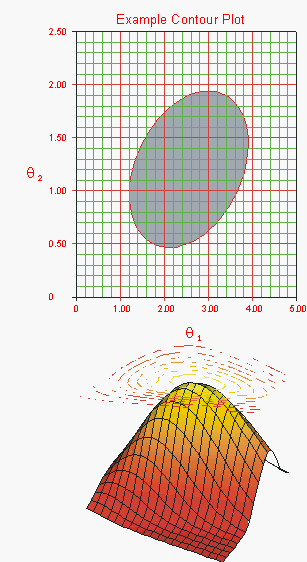
The maximum likelihood estimators (MLE) of [math]\displaystyle{ {{\theta }_{1}},{{\theta }_{2}},...,{{\theta }_{k}}, }[/math] are obtained by maximizing [math]\displaystyle{ L. }[/math] These are represented by the [math]\displaystyle{ L(\widehat{\theta }) }[/math] term in the denominator of the ratio in Eqn. (lratio1). Since the values of the data points are known, and the values of the parameter estimates [math]\displaystyle{ \widehat{\theta } }[/math] have been calculated using MLE methods, the only unknown term in Eqn. (lratio1) is the [math]\displaystyle{ L(\theta ) }[/math] term in the numerator of the ratio. It remains to find the values of the unknown parameter vector [math]\displaystyle{ \theta }[/math] that satisfy Eqn. (lratio1). For distributions that have two parameters, the values of these two parameters can be varied in order to satisfy Eqn. (lratio1). The values of the parameters that satisfy this equation will change based on the desired confidence level [math]\displaystyle{ \delta ; }[/math] but at a given value of [math]\displaystyle{ \delta }[/math] there is only a certain region of values for [math]\displaystyle{ {{\theta }_{1}} }[/math] and [math]\displaystyle{ {{\theta }_{2}} }[/math] for which Eqn. (lratio1) holds true. This region can be represented graphically as a contour plot, an example of which is given in the following graphic.
The region of the contour plot essentially represents a cross-section of the likelihood function surface that satisfies the conditions of Eqn. (lratio1).
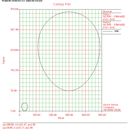
Note on Contour Plots in Weibull++ Contour plots can be used for comparing data sets. Consider two data sets, e.g. old and new design where the engineer would like to determine if the two designs are significantly different and at what confidence. By plotting the contour plots of each data set in a multiple plot (the same distribution must be fitted to each data set), one can determine the confidence at which the two sets are significantly different. If, for example, there is no overlap (i.e. the two plots do not intersect) between the two 90% contours, then the two data sets are significantly different with a 90% confidence. If there is an overlap between the two 95% contours, then the two designs are NOT significantly different at the 95% confidence level. An example of non-intersecting contours is shown next. Chapter Comparing Life Data Sets discusses comparing data sets.
Confidence Bounds on the Parameters
The bounds on the parameters are calculated by finding the extreme values of the contour plot on each axis for a given confidence level. Since each axis represents the possible values of a given parameter, the boundaries of the contour plot represent the extreme values of the parameters that satisfy:
- [math]\displaystyle{ -2\cdot \text{ln}\left( \frac{L({{\theta }_{1}},{{\theta }_{2}})}{L({{\widehat{\theta }}_{1}},{{\widehat{\theta }}_{2}})} \right)=\chi _{\alpha ;1}^{2} }[/math]
This equation can be rewritten as:
- [math]\displaystyle{ L({{\theta }_{1}},{{\theta }_{2}})=L({{\widehat{\theta }}_{1}},{{\widehat{\theta }}_{2}})\cdot {{e}^{\tfrac{-\chi _{\alpha ;1}^{2}}{2}}} }[/math]
The task now becomes to find the values of the parameters [math]\displaystyle{ {{\theta }_{1}} }[/math] and [math]\displaystyle{ {{\theta }_{2}} }[/math] so that the equality in Eqn. (lratio3) is satisfied. Unfortunately, there is no closed-form solution, thus these values must be arrived at numerically. One method of doing this is to hold one parameter constant and iterate on the other until an acceptable solution is reached. This can prove to be rather tricky, since there will be two solutions for one parameter if the other is held constant. In situations such as these, it is best to begin the iterative calculations with values close to those of the MLE values, so as to ensure that one is not attempting to perform calculations outside of the region of the contour plot where no solution exists.
Example 1 Five units were put on a reliability test and experienced failures at 10, 20, 30, 40, and 50 hours. Assuming a Weibull distribution, the MLE parameter estimates are calculated to be [math]\displaystyle{ \widehat{\beta }=2.2938 }[/math] and [math]\displaystyle{ \widehat{\eta }=33.9428. }[/math] Calculate the 90% two-sided confidence bounds on these parameters using the likelihood ratio method.
Solution to Example 1 The first step is to calculate the likelihood function for the parameter estimates:
- [math]\displaystyle{ \begin{align} L(\widehat{\beta },\widehat{\eta })= & \underset{i=1}{\overset{N}{\mathop \prod }}\,f({{x}_{i}};\widehat{\beta },\widehat{\eta })=\underset{i=1}{\overset{5}{\mathop \prod }}\,\frac{\widehat{\beta }}{\widehat{\eta }}\cdot {{\left( \frac{{{x}_{i}}}{\widehat{\eta }} \right)}^{\widehat{\beta }-1}}\cdot {{e}^{-{{\left( \tfrac{{{x}_{i}}}{\widehat{\eta }} \right)}^{\widehat{\beta }}}}} \\ \\ L(\widehat{\beta },\widehat{\eta })= & \underset{i=1}{\overset{5}{\mathop \prod }}\,\frac{2.2938}{33.9428}\cdot {{\left( \frac{{{x}_{i}}}{33.9428} \right)}^{1.2938}}\cdot {{e}^{-{{\left( \tfrac{{{x}_{i}}}{33.9428} \right)}^{2.2938}}}} \\ \\ L(\widehat{\beta },\widehat{\eta })= & 1.714714\times {{10}^{-9}} \end{align} }[/math]
where [math]\displaystyle{ {{x}_{i}} }[/math] are the original time-to-failure data points. We can now rearrange Eqn. (lratio3) to the form:
- [math]\displaystyle{ L(\beta ,\eta )-L(\widehat{\beta },\widehat{\eta })\cdot {{e}^{\tfrac{-\chi _{\alpha ;1}^{2}}{2}}}=0 }[/math]
Since our specified confidence level, [math]\displaystyle{ \delta }[/math], is 90%, we can calculate the value of the chi-squared statistic, [math]\displaystyle{ \chi _{0.9;1}^{2}=2.705543. }[/math] We then substitute this information into the equation:
- [math]\displaystyle{ \begin{align} L(\beta ,\eta )-L(\widehat{\beta },\widehat{\eta })\cdot {{e}^{\tfrac{-\chi _{\alpha ;1}^{2}}{2}}}= & 0 \\ \\ L(\beta ,\eta )-1.714714\times {{10}^{-9}}\cdot {{e}^{\tfrac{-2.705543}{2}}}= & 0 \\ \\ L(\beta ,\eta )-4.432926\cdot {{10}^{-10}}= & 0 \end{align} }[/math]
The next step is to find the set of values of [math]\displaystyle{ \beta }[/math] and [math]\displaystyle{ \eta }[/math] that satisfy this equation, or find the values of [math]\displaystyle{ \beta }[/math] and [math]\displaystyle{ \eta }[/math] such that [math]\displaystyle{ L(\beta ,\eta )=4.432926\cdot {{10}^{-10}}. }[/math]
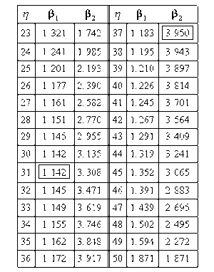
The solution is an iterative process that requires setting the value of [math]\displaystyle{ \beta }[/math] and finding the appropriate values of [math]\displaystyle{ \eta }[/math], and vice versa. The following table gives values of [math]\displaystyle{ \beta }[/math] based on given values of [math]\displaystyle{ \eta }[/math].
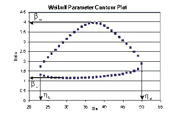
These data are represented graphically in the following contour plot:
(Note that this plot is generated with degrees of freedom [math]\displaystyle{ k=1 }[/math], as we are only determining bounds on one parameter. The contour plots generated in Weibull++ are done with degrees of freedom [math]\displaystyle{ k=2 }[/math], for use in comparing both parameters simultaneously.) As can be determined from the table, the lowest calculated value for [math]\displaystyle{ \beta }[/math] is 1.142, while the highest is 3.950. These represent the two-sided 90% confidence limits on this parameter. Since solutions for the equation do not exist for values of [math]\displaystyle{ \eta }[/math] below 23 or above 50, these can be considered the 90% confidence limits for this parameter. In order to obtain more accurate values for the confidence limits on [math]\displaystyle{ \eta }[/math], we can perform the same procedure as before, but finding the two values of [math]\displaystyle{ \eta }[/math] that correspond with a given value of [math]\displaystyle{ \beta . }[/math] Using this method, we find that the 90% confidence limits on [math]\displaystyle{ \eta }[/math] are 22.474 and 49.967, which are close to the initial estimates of 23 and 50.
Note that the points where [math]\displaystyle{ \beta }[/math] are maximized and minimized do not necessarily correspond with the points where [math]\displaystyle{ \eta }[/math] are maximized and minimized. This is due to the fact that the contour plot is not symmetrical, so that the parameters will have their extremes at different points.
Confidence Bounds on Time (Type 1)
The manner in which the bounds on the time estimate for a given reliability are calculated is much the same as the manner in which the bounds on the parameters are calculated. The difference lies in the form of the likelihood functions that comprise the likelihood ratio. In the preceding section we used the standard form of the likelihood function, which was in terms of the parameters [math]\displaystyle{ {{\theta }_{1}} }[/math] and [math]\displaystyle{ {{\theta }_{2}} }[/math]. In order to calculate the bounds on a time estimate, the likelihood function needs to be rewritten in terms of one parameter and time, so that the maximum and minimum values of the time can be observed as the parameter is varied. This process is best illustrated with an example.
Example 2
For the data given in Example 1, determine the 90% two-sided confidence bounds on the time estimate for a reliability of 50%. The ML estimate for the time at which [math]\displaystyle{ R(t)=50% }[/math] is 28.930.
Solution to Example 2
In this example, we are trying to determine the 90% two-sided confidence bounds on the time estimate of 28.930. As was mentioned, we need to rewrite Eqn. (lrbexample) so that it is in terms of [math]\displaystyle{ t }[/math] and [math]\displaystyle{ \beta . }[/math] This is accomplished by using a form of the Weibull reliability equation, [math]\displaystyle{ R={{e}^{-{{\left( \tfrac{t}{\eta } \right)}^{\beta }}}}. }[/math] This can be rearranged in terms of [math]\displaystyle{ \eta }[/math], with [math]\displaystyle{ R }[/math] being considered a known variable or:
- [math]\displaystyle{ \eta =\frac{t}{{{(-\text{ln}(R))}^{\tfrac{1}{\beta }}}} }[/math]
This can then be substituted into the [math]\displaystyle{ \eta }[/math] term in Eqn. (lrbexample) to form a likelihood equation in terms of [math]\displaystyle{ t }[/math] and [math]\displaystyle{ \beta }[/math] or:
- [math]\displaystyle{ \begin{align} & L(\beta ,t)= & \underset{i=1}{\overset{N}{\mathop \prod }}\,f({{x}_{i}};\beta ,t,R) \\ & & \end{align} }[/math]
- [math]\displaystyle{ =\underset{i=1}{\overset{5}{\mathop \prod }}\,\frac{\beta }{\left( \tfrac{t}{{{(-\text{ln}(R))}^{\tfrac{1}{\beta }}}} \right)}\cdot {{\left( \frac{{{x}_{i}}}{\left( \tfrac{t}{{{(-\text{ln}(R))}^{\tfrac{1}{\beta }}}} \right)} \right)}^{\beta -1}}\cdot \text{exp}\left[ -{{\left( \frac{{{x}_{i}}}{\left( \tfrac{t}{{{(-\text{ln}(R))}^{\tfrac{1}{\beta }}}} \right)} \right)}^{\beta }} \right] }[/math]
where [math]\displaystyle{ {{x}_{i}} }[/math] are the original time-to-failure data points. We can now rearrange Eqn. (lratio3) to the form:
- [math]\displaystyle{ L(\beta ,t)-L(\widehat{\beta },\widehat{\eta })\cdot {{e}^{\tfrac{-\chi _{\alpha ;1}^{2}}{2}}}=0 }[/math]
Since our specified confidence level, [math]\displaystyle{ \delta }[/math], is 90%, we can calculate the value of the chi-squared statistic, [math]\displaystyle{ \chi _{0.9;1}^{2}=2.705543. }[/math] We can now substitute this information into the equation:
- [math]\displaystyle{ \begin{align} L(\beta ,t)-L(\widehat{\beta },\widehat{\eta })\cdot {{e}^{\tfrac{-\chi _{\alpha ;1}^{2}}{2}}}= & 0 \\ \\ L(\beta ,t)-1.714714\times {{10}^{-9}}\cdot {{e}^{\tfrac{-2.705543}{2}}}= & 0 \\ & \\ L(\beta ,t)-4.432926\cdot {{10}^{-10}}= & 0 \end{align} }[/math]
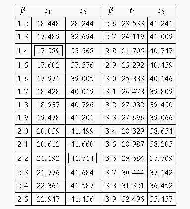
Note that the likelihood value for [math]\displaystyle{ L(\widehat{\beta },\widehat{\eta }) }[/math] is the same as it was for Example 1. This is because we are dealing with the same data and parameter estimates or, in other words, the maximum value of the likelihood function did not change. It now remains to find the values of [math]\displaystyle{ \beta }[/math] and [math]\displaystyle{ t }[/math] which satisfy this equation. This is an iterative process that requires setting the value of [math]\displaystyle{ \beta }[/math] and finding the appropriate values of [math]\displaystyle{ t }[/math]. The following table gives the values of [math]\displaystyle{ t }[/math] based on given values of [math]\displaystyle{ \beta }[/math].
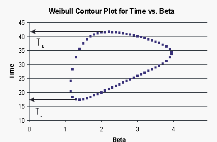
These points are represented graphically in the following contour plot:
As can be determined from the table, the lowest calculated value for [math]\displaystyle{ t }[/math] is 17.389, while the highest is 41.714. These represent the 90% two-sided confidence limits on the time at which reliability is equal to 50%.
Confidence Bounds on Reliability (Type 2)
The likelihood ratio bounds on a reliability estimate for a given time value are calculated in the same manner as were the bounds on time. The only difference is that the likelihood function must now be considered in terms of [math]\displaystyle{ \beta }[/math] and [math]\displaystyle{ R }[/math]. The likelihood function is once again altered in the same way as before, only now [math]\displaystyle{ R }[/math] is considered to be a parameter instead of [math]\displaystyle{ t }[/math], since the value of [math]\displaystyle{ t }[/math] must be specified in advance. Once again, this process is best illustrated with an example.
Example 3 For the data given in Example 1, determine the 90% two-sided confidence bounds on the reliability estimate for [math]\displaystyle{ t=45 }[/math]. The ML estimate for the reliability at [math]\displaystyle{ t=45 }[/math] is 14.816%.
Solution to Example 3 In this example, we are trying to determine the 90% two-sided confidence bounds on the reliability estimate of 14.816%. As was mentioned, we need to rewrite Eqn. (lrbexample) so that it is in terms of [math]\displaystyle{ R }[/math] and [math]\displaystyle{ \beta . }[/math] This is again accomplished by substituting the Weibull reliability equation into the [math]\displaystyle{ \eta }[/math] term in Eqn. (lrbexample) to form a likelihood equation in terms of [math]\displaystyle{ R }[/math] and [math]\displaystyle{ \beta }[/math]:
- [math]\displaystyle{ \begin{align} & L(\beta ,R)= & \underset{i=1}{\overset{N}{\mathop \prod }}\,f({{x}_{i}};\beta ,t,R) \\ & & \end{align} }[/math]
- [math]\displaystyle{ =\underset{i=1}{\overset{5}{\mathop \prod }}\,\frac{\beta }{\left( \tfrac{t}{{{(-\text{ln}(R))}^{\tfrac{1}{\beta }}}} \right)}\cdot {{\left( \frac{{{x}_{i}}}{\left( \tfrac{t}{{{(-\text{ln}(R))}^{\tfrac{1}{\beta }}}} \right)} \right)}^{\beta -1}}\cdot \text{exp}\left[ -{{\left( \frac{{{x}_{i}}}{\left( \tfrac{t}{{{(-\text{ln}(R))}^{\tfrac{1}{\beta }}}} \right)} \right)}^{\beta }} \right] }[/math]
where [math]\displaystyle{ {{x}_{i}} }[/math] are the original time-to-failure data points. We can now rearrange Eqn. (lratio3) to the form:
- [math]\displaystyle{ L(\beta ,R)-L(\widehat{\beta },\widehat{\eta })\cdot {{e}^{\tfrac{-\chi _{\alpha ;1}^{2}}{2}}}=0 }[/math]
Since our specified confidence level, [math]\displaystyle{ \delta }[/math], is 90%, we can calculate the value of the chi-squared statistic, [math]\displaystyle{ \chi _{0.9;1}^{2}=2.705543. }[/math] We can now substitute this information into the equation:
- [math]\displaystyle{ \begin{align} L(\beta ,R)-L(\widehat{\beta },\widehat{\eta })\cdot {{e}^{\tfrac{-\chi _{\alpha ;1}^{2}}{2}}}= & 0 \\ \\ L(\beta ,R)-1.714714\times {{10}^{-9}}\cdot {{e}^{\tfrac{-2.705543}{2}}}= & 0 \\ \\ L(\beta ,R)-4.432926\cdot {{10}^{-10}}= & 0 \end{align} }[/math]
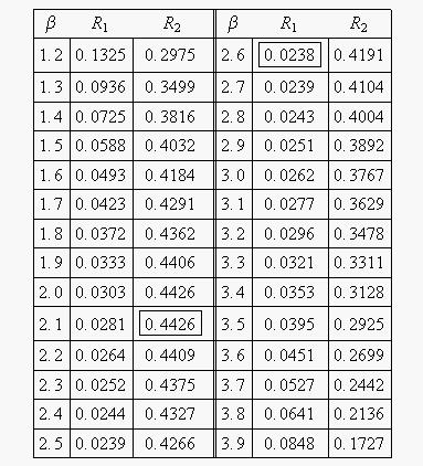
It now remains to find the values of [math]\displaystyle{ \beta }[/math] and [math]\displaystyle{ R }[/math] that satisfy this equation. This is an iterative process that requires setting the value of [math]\displaystyle{ \beta }[/math] and finding the appropriate values of [math]\displaystyle{ R }[/math]. The following table gives the values of [math]\displaystyle{ R }[/math] based on given values of [math]\displaystyle{ \beta }[/math].
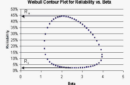
These points are represented graphically in the following contour plot:
As can be determined from the table, the lowest calculated value for [math]\displaystyle{ R }[/math] is 2.38%, while the highest is 44.26%. These represent the 90% two-sided confidence limits on the reliability at [math]\displaystyle{ t=45 }[/math].
