Template:Testing methodology rga: Difference between revisions
(Created page with '==Testing Methodology== The methodology described here will use the Crow Extended model (presented in Chapter 9) for data analysis. In order to have valid Crow Extended model ass…') |
Lisa Hacker (talk | contribs) |
||
| Line 6: | Line 6: | ||
<br> | <br> | ||
<br> | <br> | ||
==Example== | |||
Consider the test-fix-find-test data of Example 2 in Chapter 9, which is shown again in Table 12.1. The total test time for this test is 400 hours. Note that for this example we assume one stopping point at the end of the test for the incorporation of the delayed fixes. Suppose that the data set represents a military system with Task 1 firing a gun, Task 2 moving under environment E1 and Task 3 moving under environment E2. For every hour of operation the operational profile states that the system operates in environment E1 70% of the time and in environment E2 30% of the time. In addition, for each hour of operation the gun must be fired 10 times. | Consider the test-fix-find-test data of Example 2 in Chapter 9, which is shown again in Table 12.1. The total test time for this test is 400 hours. Note that for this example we assume one stopping point at the end of the test for the incorporation of the delayed fixes. Suppose that the data set represents a military system with Task 1 firing a gun, Task 2 moving under environment E1 and Task 3 moving under environment E2. For every hour of operation the operational profile states that the system operates in environment E1 70% of the time and in environment E2 30% of the time. In addition, for each hour of operation the gun must be fired 10 times. | ||
<br> | <br> | ||
Revision as of 00:46, 23 August 2012
Testing Methodology
The methodology described here will use the Crow Extended model (presented in Chapter 9) for data analysis. In order to have valid Crow Extended model assessments, it is required that the operational mission profile be conducted in a structured manner. Therefore, this testing methodology involves convergence and stopping points during the testing. A stopping point is when the testing is stopped for the expressed purpose of incorporating the Type BD delayed corrective actions. There may be more than one stopping point during a particular testing phase. For simplicity, the methodology with only one stopping point will be described; however, the methodology can be extended to the case of more than one stopping point. A convergence point is a time during the test when all the operational mission profile tasks meet their expected averages or fall within an acceptable range. At least three convergence points are required for a well-balanced test. The end of the test, time [math]\displaystyle{ T }[/math] , must be a convergence point. The test times between the convergence points do not have to be the same.
The objective of having the convergence points is to be able to apply the Crow Extended model directly in such a way that the projection and other key reliability growth parameters can be estimated in a valid fashion. To do this, the grouped data methodology is applied. Note that the methodology also can be used with the Crow-AMSAA (NHPP) model for a simpler analysis without the ability to estimate projected and growth potential reliability. For the Crow-AMSAA (NHPP) grouped data methodology, refer to Chapter 5, Section 3. For grouped data using the Crow Extended model, refer to Chapter 9, Section 6.
Example
Consider the test-fix-find-test data of Example 2 in Chapter 9, which is shown again in Table 12.1. The total test time for this test is 400 hours. Note that for this example we assume one stopping point at the end of the test for the incorporation of the delayed fixes. Suppose that the data set represents a military system with Task 1 firing a gun, Task 2 moving under environment E1 and Task 3 moving under environment E2. For every hour of operation the operational profile states that the system operates in environment E1 70% of the time and in environment E2 30% of the time. In addition, for each hour of operation the gun must be fired 10 times.
In general, it is difficult to manage an operational test so that these operational profiles are continuously met throughout the test. However, the operational mission profile methodology requires that these conditions be met on average at the convergence points. In practice, this almost always can be done with proper program and test management. The convergence points are set for the testing, often at interim assessment points. The process for controlling the convergence at these points involves monitoring a graph for each of the tasks.
Table 12.2 shows the expected and actual results for each of the operational mission profiles.
| Table 12.1 - Test-fix-find-test data | ||||||
| [math]\displaystyle{ i }[/math] | [math]\displaystyle{ {{X}_{i}} }[/math] | Mode | [math]\displaystyle{ i }[/math] | [math]\displaystyle{ {{X}_{i}} }[/math] | Mode | |
|---|---|---|---|---|---|---|
| 1 | 0.7 | BC17 | 29 | 192.7 | BD11 | |
| 2 | 3.7 | BC17 | 30 | 213 | A | |
| 3 | 13.2 | BC17 | 31 | 244.8 | A | |
| 4 | 15 | BD1 | 32 | 249 | BD12 | |
| 5 | 17.6 | BC18 | 33 | 250.8 | A | |
| 6 | 25.3 | BD2 | 34 | 260.1 | BD1 | |
| 7 | 47.5 | BD3 | 35 | 263.5 | BD8 | |
| 8 | 54 | BD4 | 36 | 273.1 | A | |
| 9 | 54.5 | BC19 | 37 | 274.7 | BD6 | |
| 10 | 56.4 | BD5 | 38 | 282.8 | BC27 | |
| 11 | 63.6 | A | 39 | 285 | BD13 | |
| 12 | 72.2 | BD5 | 40 | 304 | BD9 | |
| 13 | 99.2 | BC20 | 41 | 315.4 | BD4 | |
| 14 | 99.6 | BD6 | 42 | 317.1 | A | |
| 15 | 100.3 | BD7 | 43 | 320.6 | A | |
| 16 | 102.5 | A | 44 | 324.5 | BD12 | |
| 17 | 112 | BD8 | 45 | 324.9 | BD10 | |
| 18 | 112.2 | BC21 | 46 | 342 | BD5 | |
| 19 | 120.9 | BD2 | 47 | 350.2 | BD3 | |
| 20 | 121.9 | BC22 | 48 | 355.2 | BC28 | |
| 21 | 125.5 | BD9 | 49 | 364.6 | BD10 | |
| 22 | 133.4 | BD10 | 50 | 364.9 | A | |
| 23 | 151 | BC23 | 51 | 366.3 | BD2 | |
| 24 | 163 | BC24 | 52 | 373 | BD8 | |
| 25 | 164.7 | BD9 | 53 | 379.4 | BD14 | |
| 26 | 174.5 | BC25 | 54 | 389 | BD15 | |
| 27 | 177.4 | BD10 | 55 | 394.9 | A | |
| 28 | 191.6 | BC26 | 56 | 395.2 | BD16 | |
| Table 12.2 - Expected and actual results for profiles 1, 2, 3 | ||||||
| Profile 1(gun firings) | Profile 2(E1) | Profile 3(E2) | ||||
| Time | Expected | Actual | Expected | Actual | Expected | Actual |
| 5 | 50 | 0 | 3.5 | 5 | 1.5 | 0 |
| 10 | 100 | 0 | 7 | 10 | 3 | 0 |
| 15 | 150 | 0 | 10.5 | 15 | 4.5 | 0 |
| 20 | 200 | 0 | 14 | 20 | 6 | 0 |
| 25 | 250 | 100 | 17.5 | 25 | 7.5 | 0 |
| 30 | 300 | 150 | 21 | 30 | 9 | 0 |
| 35 | 350 | 400 | 24.5 | 30 | 10.5 | 5 |
| 40 | 400 | 600 | 28 | 30 | 12 | 10 |
| 45 | 450 | 600 | 31.5 | 30 | 13.5 | 15 |
| 50 | 500 | 600 | 35 | 30 | 15 | 20 |
| 55 | 550 | 800 | 38.5 | 35 | 16.5 | 20 |
| 60 | 600 | 800 | 42 | 40 | 18 | 20 |
| 65 | 650 | 800 | 45.5 | 45 | 19.5 | 20 |
| 70 | 700 | 800 | 49 | 50 | 21 | 20 |
| 75 | 750 | 800 | 52.5 | 55 | 22.5 | 20 |
| 80 | 800 | 900 | 56 | 55 | 24 | 25 |
| 85 | 850 | 950 | 59.5 | 55 | 25.5 | 30 |
| 90 | 900 | 1000 | 63 | 60 | 27 | 30 |
| 95 | 950 | 1000 | 66.5 | 65 | 28.5 | 30 |
| 100 | 1000 | 1000 | 70 | 70 | 30 | 30 |
| 105 | 1050 | 1000 | 73.5 | 70 | 31.5 | 35 |
| ... | ... | ... | ... | ... | ... | |
| ... | ... | ... | ... | ... | ... | |
| 355 | 3550 | 3440 | 248.5 | 259 | 106.5 | 96 |
| 360 | 3600 | 3690 | 252 | 264 | 108 | 96 |
| 365 | 3650 | 3690 | 255.5 | 269 | 109.5 | 96 |
| 370 | 3700 | 3850 | 259 | 274 | 111 | 96 |
| 375 | 3750 | 3850 | 262.5 | 279 | 112.5 | 96 |
| 380 | 3800 | 3850 | 266 | 280 | 114 | 100 |
| 385 | 3850 | 3850 | 269.5 | 280 | 115.5 | 105 |
| 390 | 3900 | 3850 | 273 | 280 | 117 | 110 |
| 395 | 3950 | 4000 | 276.5 | 280 | 118.5 | 115 |
| 400 | 4000 | 4000 | 280 | 280 | 120 | 120 |
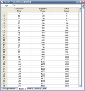
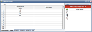
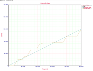
Figure Profile shows a portion of the expected and actual results for mission profile 1, as entered in RGA 7. A graph exists for each of the three tasks in this example. Each graph has a line with the expected average as a function of hours, and the corresponding actual value. When the actual value for a task meets the expected value then is a convergence for that task. A convergence point occurs when all of the tasks converge at the same time. At least three convergence points are required, one of which is the stopping point [math]\displaystyle{ T }[/math] . In our example, the total test time is 400 hours. The convergence points were chosen to be at 100, 250, 320 and 400 hours. Figure convergence points shows the data sheet that contains the convergence points in RGA 7.
[math]\displaystyle{ }[/math]
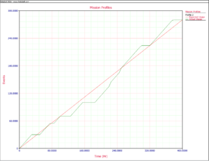
The testing profiles are managed so that at these times the actual operational test profile equals the expected values for the three tasks or falls within an acceptable range. Figure firings shows the expected and actual gun firings. Figure E1 shows the expected and actual time in environment E1 and Figure E2 shows the expected and actual time in environment E2.
[math]\displaystyle{ }[/math]
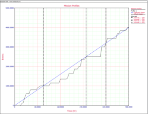
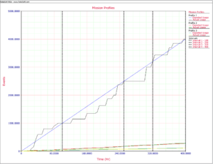
The objective of having the convergence points is to be able to apply the Crow Extended model directly in such a way that the projection and other key reliability growth parameters can be estimated in a valid fashion. To do this, grouped data is applied using the Crow Extended model. For reliability growth assessments using grouped data, only information between time points in the testing is used. In our application, these time points are the convergence points: 100, 250, 320, and 400. Figure Combinedission shows all three mission profiles plotted in the same graph, together with the convergence points.
Table 12.3 gives the grouped data input corresponding to the data in Table 12.1.
The parameters of the Crow Extended model for grouped data are then estimated, as explained in Chapter 9, Section 6. Table 12.4 shows the effectiveness factors (EFs) for each of the BD modes.
| Table 12.3 - Grouped data at convergence points 100, 250, 320 and 400 hours | ||||||||
| Number at Event | Time to Event | Classification | Mode | Number at Event | Time to Event | Classification | Mode | |
|---|---|---|---|---|---|---|---|---|
| 3 | 100 | BC | 17 | 1 | 250 | BC | 26 | |
| 1 | 100 | BD | 1 | 1 | 250 | BD | 11 | |
| 1 | 100 | BC | 18 | 1 | 250 | BD | 12 | |
| 1 | 100 | BD | 2 | 3 | 320 | A | ||
| 1 | 100 | BD | 3 | 1 | 320 | BD | 1 | |
| 1 | 100 | BD | 4 | 1 | 320 | BD | 8 | |
| 1 | 100 | BC | 19 | 1 | 320 | BD | 6 | |
| 2 | 100 | BD | 5 | 1 | 320 | BC | 27 | |
| 1 | 100 | A | 1 | 320 | BD | 13 | ||
| 1 | 100 | BC | 20 | 1 | 320 | BD | 9 | |
| 1 | 100 | BD | 6 | 1 | 320 | BD | 4 | |
| 1 | 250 | BD | 7 | 3 | 400 | A | ||
| 3 | 250 | A | 1 | 400 | BD | 12 | ||
| 1 | 250 | BD | 8 | 2 | 400 | BD | 10 | |
| 1 | 250 | BC | 21 | 1 | 400 | BD | 5 | |
| 1 | 250 | BD | 2 | 1 | 400 | BD | 3 | |
| 1 | 250 | BC | 22 | 1 | 400 | BC | 28 | |
| 2 | 250 | BD | 9 | 1 | 400 | BD | 2 | |
| 2 | 250 | BD | 10 | 1 | 400 | BD | 8 | |
| 1 | 250 | BC | 23 | 1 | 400 | BD | 14 | |
| 1 | 250 | BC | 24 | 1 | 400 | BD | 15 | |
| 1 | 250 | BC | 25 | 1 | 400 | BD | 16 | |
| Table 12.4 - Effectiveness Factors for delayed fixes | |
| Mode | Effectiveness Factor |
|---|---|
| 1 | 0.67 |
| 2 | 0.72 |
| 3 | 0.77 |
| 4 | 0.77 |
| 5 | 0.87 |
| 6 | 0.92 |
| 7 | 0.50 |
| 8 | 0.85 |
| 9 | 0.89 |
| 10 | 0.74 |
| 11 | 0.70 |
| 12 | 0.63 |
| 13 | 0.64 |
| 14 | 0.72 |
| 15 | 0.69 |
| 16 | 0.46 |
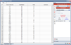
Using the Crow Extended failure times Data Sheet shown in Figure Failure times data, we can analyze this data set based on a mission profile by clicking the mission profile icon:
[math]\displaystyle{ }[/math]
[math]\displaystyle{ }[/math]
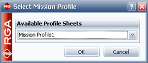
A specific mission profile can then be associated with the Data Sheet, as shown in Figure selecting. This will group the failure times data into groups based on the convergence points that have already been specified when constructing the mission profile.
[math]\displaystyle{ }[/math]
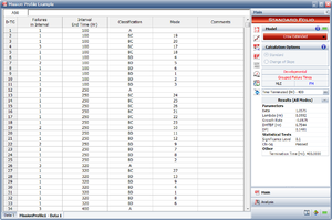
A new data sheet with the grouped data is created, as shown in Figure groupedata.
The calculated results based on the grouped data are as follows:
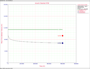
Figure growth potential shows the instantaneous, demonstrated, projected and growth potential MTBF for the grouped data, based the mission profile grouping with intervals at the specified convergence points of the mission profile.
