Availability Analysis Reference Example: Difference between revisions
Jump to navigation
Jump to search
Kate Racaza (talk | contribs) No edit summary |
Kate Racaza (talk | contribs) No edit summary |
||
| (One intermediate revision by the same user not shown) | |||
| Line 10: | Line 10: | ||
{{Reference_Example_Heading2}} | {{Reference_Example_Heading2}} | ||
A two-component system’s point and interval availability for a 10 hour mission and the steady-state availability for both series and parallel configurations are calculated. The components share the same failure rate and repair rate distributions. The failure and repair rates both follow exponential distributions with a failure rate of 0.1 failures per hour and a repair rate of 0.2 repairs per hour. | A two-component system’s point and interval availability for a 10 hour mission, and the steady-state availability for both series and parallel configurations are calculated. The components share the same failure rate and repair rate distributions. The failure and repair rates both follow exponential distributions with a failure rate of 0.1 failures per hour and a repair rate of 0.2 repairs per hour. | ||
{| {{Table}} | {| {{Table}} | ||
| Line 35: | Line 35: | ||
The system availability for ''n'' independent components in series, each having a component availability of <math> A_{ | The system availability for ''n'' independent components in series, each having a component availability of <math> A_{i}(t)\,\!</math>, is given in Equation 11.15 on page 259 in the reference book as: | ||
::<math>A_{s}(t) = \prod _{i=1}^{n}A_{i}(t)\,\!</math> | ::<math>A_{s}(t) = \prod _{i=1}^{n}A_{i}(t)\,\!</math> | ||
The system availability for ''n'' independent components in parallel, each having a component availability of <math> A_{ | The system availability for ''n'' independent components in parallel, each having a component availability of <math> A_{i}(t)\,\!</math>, is given in Equation 11.16 on page 259 in the reference book as: | ||
::<math>A_{s}(t) = 1- \prod _{i=1}^{n}(1-A_{i}(t))\,\!</math> | ::<math>A_{s}(t) = 1- \prod _{i=1}^{n}(1-A_{i}(t))\,\!</math> | ||
| Line 66: | Line 66: | ||
{{Reference_Example_Heading4|BlockSim}} | {{Reference_Example_Heading4|BlockSim}} | ||
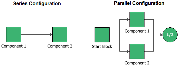
In BlockSim, the system RBDs are configured as shown below for series and parallel configurations. Since this is an availability example, we will validate the results via simulation. | In BlockSim, the system RBDs are configured as shown below for series and parallel configurations. Since this is an availability example, we will validate the results via simulation. | ||
| Line 72: | Line 72: | ||
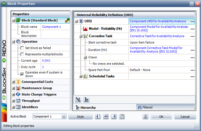
Each component is modeled using a 1-parameter exponential distribution with the given lambda (failure rate) values. They also share a corrective task that is modeled | Each component is modeled using a 1-parameter exponential distribution with the given lambda (failure rate) values. They also share a corrective task that is modeled using a 1-parameter exponential distribution with the given lambda (repair rate) values. In this example, we are assuming that the component is fixed upon item failure to as good as new condition. One important point to keep in mind is that the component that is not failed still accumulates time while the corrective task is taking place for the component that failed. The reference book follows this assumption while driving the equations given above. | ||
[[Image:availability_properties.png|center]] | [[Image:availability_properties.png|center|650px]] | ||
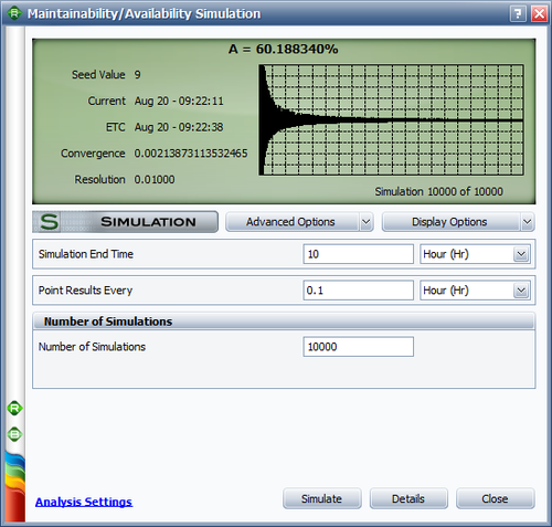
The same simulation setup is used for both series and parallel configurations. | The same simulation setup is used for both series and parallel configurations. To estimate the point and interval availability for a 10 hour mission, we use a simulation end time of 10 hours. The settings are shown next. | ||
[[Image:availability_sim.png|center]] | [[Image:availability_sim.png|center|500px]] | ||
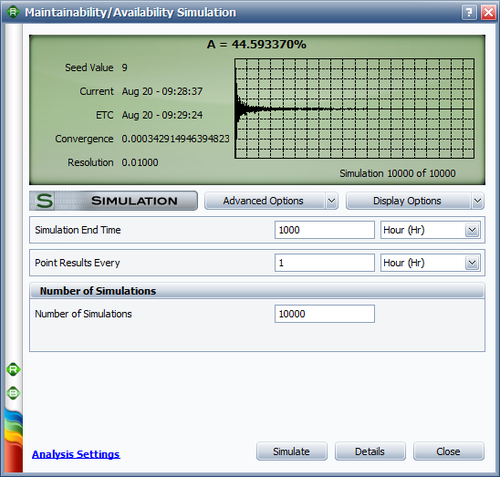
To estimate the steady-state availability, we use a simulation end time of 1,000 hours, since the system is assumed to reach steady state at that time. The settings are shown next. | |||
[[Image:availability_sim2.png|center|500px]] | |||
| Line 100: | Line 105: | ||
A_{s} &= 0.8893\\ | A_{s} &= 0.8893\\ | ||
\end{align}\,\!</math> | \end{align}\,\!</math> | ||
Latest revision as of 16:35, 20 August 2015
New format available! This reference is now available in a new format that offers faster page load, improved display for calculations and images and more targeted search.
As of January 2024, this Reliawiki page will not continue to be updated. Please update all links and bookmarks to the latest references at BlockSim examples and BlockSim reference examples.


