Robust Parameter Design: Difference between revisions
| (78 intermediate revisions by 5 users not shown) | |||
| Line 1: | Line 1: | ||
{{Template:Doebook| | {{Template:Doebook|13}} | ||
In [[Response_Surface_Methods_for_Optimization|Response Surface Methods for Optimization]], techniques used to optimize the response were discussed. Once an optimum value of the response has been achieved, the next goal of the experimenter should be to make the optimum response value insensitive to the noise factors so that a consistent performance is obtained at all times. For example, if the yield from a chemical process has been optimized at 95%, then this value of yield should be obtained regardless of the variation in factors such as the quality of reactants or fluctuations in humidity or other weather conditions. These factors are beyond the control of the operator. Therefore, the product or process should be such that it is not affected by minor fluctuations in these factors. The process of making a system insensitive to such factors is referred to as ''robust design''. Robust design was pioneered by the Japanese industrialist Dr. Genichi Taguchi in the early 1980s. This chapter briefly discusses his approach. | |||
==Taguchi's Philosophy== | |||
Taguchi's philosophy is based on the fact that any decrease in the quality of a system leads to customer dissatisfaction. This occurs even if the departure in quality lies within the specified limits of the system and is considered acceptable to the customer. For example, consider the case of a laptop that develops a defect on its screen within the warranty period. Although the customer is able to get a warranty-replacement for the screen this might lead to a little dissatisfaction on the part of the customer. If the same laptop then develops a problem with its DVD drive, the customer might declare the laptop "useless," even if the problem occurs during the warranty period and the customer is able to get a free replacement. Therefore, to maintain a good reputation, the laptop manufacturer needs to produce laptops that offer the same quality to all customers consistently. This can only be done when the required quality is built into the laptops. Note how this approach differs from traditional quality control where it is considered sufficient to manufacture products within certain specifications and carry out pre-shipment quality control inspections (i.e., sampling inspections) to filter out products that fall out of specification. | |||
Taguchi's philosophy requires that systems be designed in such a way that they are produced, not just within the specified limits, but right on target specifications or best values. Such a proactive approach is much more fruitful and efficient than the reactive approach of sampling inspections. The philosophy of Taguchi is summarized by his quality loss function (see the figure below). The function states that any deviation from the target value leads to a quadratic loss in quality or customer satisfaction. Mathematically, the function may be expressed as: | |||
::<math>L=k{{(y-m)}^{2}}\,\!</math> | |||
[[Image:doe10.1.png|center|337px|Taguchi's quality loss function.|link=]] | |||
<math> | where <math>y\,\!</math> represents the performance parameter of the system, <math>m\,\!</math> represents the target or the nominal value of <math>y\,\!</math>, <math>L\,\!</math> represents the quality loss and <math>k\,\!</math> is a constant. | ||
< | |||
< | |||
< | |||
< | |||
Taguchi's approach to achieve a high quality system consists of three stages: ''system design'', ''parameter design'' and ''tolerance design''. System design refers to the stage when ideas for a new system are used to decide upon the combinations of factors to obtain a functional and economical design. Parameter design refers to the stage when factor settings are selected that make the system less sensitive to variations in the uncontrollable factors affecting the system. Therefore, if this stage is carried out successfully, the resulting system will have little variation and the resulting tolerances will be tight. Tolerance design refers to the final stage when tolerances are tightened around the best value. This stage increases cost and is only needed if the required quality is not achieved during parameter design. Thus, using parameter design, it is possible to achieve the desired quality without much increase in the cost. The tolerance design stage is discussed in detail next. | |||
Taguchi's approach to achieve a high quality system consists of three stages | |||
==Robust Parameter Design== | ==Robust Parameter Design== | ||
Taguchi divided the factors affecting any system into two categories | Taguchi divided the factors affecting any system into two categories: ''control factors'' and ''noise factors''. Control factors are factors affecting a system that are easily set by the experimenter. For example, if in a chemical process the reaction time is found to be a factor affecting the yield, then this factor is a control factor since it can be easily manipulated and set by the experimenter. The experimenter will chose the setting of the reaction time that maximizes the yield. Noise factors are factors affecting a system that are difficult or impossible to control. For example, ambient temperature may also have an effect on the yield of a chemical process, but ambient temperature could be a noise factor if it is beyond the control of the experimenter. Thus, change in ambient temperature will lead to variations in the yield but such variations are undesirable. | ||
===Control and Noise Factor Interaction=== | ===Control and Noise Factor Interaction=== | ||
In our example, since the experimenter does not have any control on the change in ambient temperature, he/she needs to find the setting of the reaction time at which there is minimal variation of yield due to change in ambient temperature. Note that this can only occur if there is an interaction between the reaction time (control factor) and ambient temperature (noise factor). If there is no such interaction, variation in yield due to changes in ambient temperature will always occur regardless of the setting of the reaction time. Therefore, to solve a robust parameter design problem, interaction between control and noise factors must exist. This fact is further explained by | In our example, since the experimenter does not have any control on the change in ambient temperature, he/she needs to find the setting of the reaction time at which there is minimal variation of yield due to change in ambient temperature. Note that this can only occur if there is an interaction between the reaction time (control factor) and ambient temperature (noise factor). If there is no such interaction, variation in yield due to changes in ambient temperature will always occur regardless of the setting of the reaction time. Therefore, to solve a robust parameter design problem, interaction between control and noise factors must exist. This fact is further explained by the figure shown next. | ||
[[Image:doe10.2.png|center|324px|Interaction between control and noise factors: (a) shows the case when there is no such interaction and (b) shows the case when the interaction exists. Robust design is only possible in case (b).|link=]] | |||
The figure shows the variation of the response (yield) for two levels of the noise factor (ambient temperature). The response values are plotted at two levels of the control factor (reaction time). Figure (a) shows the case where there is no interaction between the control and noise factors. It can be seen that, regardless of the settings of the control factor (low or high), the variation in the response remains the same (as is evident from the constant spread of the probability distribution of the response at the two levels of the control factor). Figure (b) shows the case where an interaction exists between the control and noise factors. The figure indicates that in the present case it is advantageous to have the control factor at the low setting, since at this setting there is not much variation in the response due to change in the noise factor (as is evident from the smaller spread of the probability distribution of the response at the low level of the control factor). | |||
===Inner and Outer Arrays=== | ===Inner and Outer Arrays=== | ||
Taguchi studied the interaction between the control and noise factors using two experiment designs | Taguchi studied the interaction between the control and noise factors using two experiment designs: the ''inner array'' and the ''outer array''. The inner array is essentially any experiment design that is used to study the effect of the control factors on the response. Taguchi then used an outer array for the noise factors so that each run of the inner array was repeated for every treatment of the outer array. The resulting experiment design, that uses both inner and outer arrays, is referred to as a ''cross array''. | ||
====Example==== | |||
To illustrate Taguchi's use of the inner and outer arrays consider the case of a chemical process where the experimenter wants the product to be neither acidic nor basic (i.e., the pH of the product needs to be as close to 7 as possible). It is thought that the pH of the product depends on the concentration of the three reactants, <math>A\,\!</math>, <math>B\,\!</math> and <math>C\,\!</math>, used to obtain the product. There are three control factors here, namely the concentration of each of the three reactants. It has also been found that the pH of the product depends on the ambient temperature which varies naturally and cannot be controlled. Thus, there is one noise factor in this case - the ambient temperature. The experimenter chooses Taguchi's robust parameter design approach to investigate the settings of the control factors to make the product insensitive to changes in ambient temperature. It is decided to carry out a <math>2^{3}\,\!</math> experiment to study the effect of the three control factors on the pH of the product. Therefore, the <math>2^{3}\,\!</math> design is the inner array here. It is also decided to carry out the experiment at four levels of the ambient temperature by using a special enclosure where the surrounding temperature of the chemical process can be controlled. Therefore, the outer array consists of a single factor experiment with the factor at four levels. Note that, in order to carry out the robust parameter design approach, the noise factor should be such that it can be controlled in an experimental setting. The resulting setup of the robust parameter design experiment is shown in the following table. | |||
To illustrate Taguchi's use of the inner and outer arrays consider the case of a chemical process where the experimenter wants the product to be neither acidic nor basic (i.e. the pH of the product needs to be as close to 7 as possible). It is thought that the pH of the product depends on the concentration of the three reactants, | |||
[[Image:doet10.1.png|center|462px|Data for the experiment in the example.|link=]] | |||
<math></math> | The experiment requires <math>2^{3}\times 4=32\,\!</math> runs in all as each run of the inner array is repeated for every treatment of the outer array. The above table also shows the pH values obtained for the experiment. In a Weibull++ DOE folio, this design is set up by specifying the properties for the inner and outer arrays as shown in the following figure. | ||
[[Image:doe13_1.png|center|575px|Design properties for the factors in the example.|link=]] | |||
The resulting design is shown in the next figure. | |||
[[Image:doe13_2.png|center|550px|Cross array design for the example.|link=]] | |||
==Signal to Noise Ratios== | ==Signal to Noise Ratios== | ||
Depending upon the objective of the robust parameter design, Taguchi defined three different statistics called signal to noise ratios. These ratios were defined as the means to measure the variation of the response with respect to the noise factors. Taguchi's approach essentially consists of two models | Depending upon the objective of the robust parameter design, Taguchi defined three different statistics called ''signal to noise ratios''. These ratios were defined as the means to measure the variation of the response with respect to the noise factors. Taguchi's approach essentially consists of two models: a ''location model'' and a ''dispersion model''. | ||
===Location Model=== | ===Location Model=== | ||
The location model is the regression model for the mean value of the response at each treatment combination of the inner array. If | The location model is the regression model for the mean value of the response at each treatment combination of the inner array. If <math>{{y}_{ij}}\,\!</math> (<math>j=1\,\!</math> <math>to\,\!</math> <math>m\,\!</math>) represents the <math>m\,\!</math> response values obtained at the <math>i\,\!</math>th treatment combination of the inner array (corresponding to the <math>m\,\!</math> levels of the noise factors), then the mean response at the <math>i\,\!</math>th level is: | ||
<math>{{\bar{y}}_{i}}=\frac{1}{m}\underset{j=1}{\overset{m}{\mathop \sum }}\,{{y}_{ij}}</math> | |||
::<math>{{\bar{y}}_{i}}=\frac{1}{m}\underset{j=1}{\overset{m}{\mathop \sum }}\,{{y}_{ij}}\,\!</math> | |||
The location model is obtained by fitting a regression model to all <math>{{\bar{y}}_{i}}\,\!</math> values, by treating these values as the response at each of the <math>i\,\!</math>th treatments of the inner array. As an example, the location model for an inner array with two factors can be written as: | |||
<math>{{\bar{y}}_{i}}=\beta _{0}^{L}+\beta _{1}^{L}{{x}_{i1}}+\beta _{2}^{L}{{x}_{i2}}+\beta _{12}^{L}{{x}_{i1}}{{x}_{i2}}</math> | ::<math>{{\bar{y}}_{i}}=\beta _{0}^{L}+\beta _{1}^{L}{{x}_{i1}}+\beta _{2}^{L}{{x}_{i2}}+\beta _{12}^{L}{{x}_{i1}}{{x}_{i2}}\,\!</math> | ||
where: | where: | ||
*<math>\beta _{0}^{L}\,\!</math> is the intercept | |||
*<math>\beta _{1}^{L}\,\!</math> is the coefficient for the first factor | |||
*<math>\beta _{2}^{L}\,\!</math> is the coefficient for the second factor | |||
The objective of using the location model is to bring the response to its goal regardless of whether this is a target value, maximum value or minimum value. This is done by identifying significant effects and then using the least square estimates of the corresponding coefficients, | *<math>\beta _{12}^{L}\,\!</math> is the coefficient for the interaction | ||
*<math>{{x}_{1}}\,\!</math> and <math>{{x}_{2}}\,\!</math> are respectively the variables for the two factors | |||
The objective of using the location model is to bring the response to its goal regardless of whether this is a target value, maximum value or minimum value. This is done by identifying significant effects and then using the least square estimates of the corresponding coefficients, <math>{{\beta }^{L}}\,\!</math>s, to fit the location model. The fitted model is used to decide the settings of the variables that bring the response to the goal. | |||
===Dispersion Model=== | ===Dispersion Model=== | ||
The dispersion model measures the variation of the response due to the noise factors. The standard deviation of the response values at each treatment combination, | The dispersion model measures the variation of the response due to the noise factors. The standard deviation of the response values at each treatment combination, <math>{{s}_{i}}\,\!</math>, is used. Usually, the standard deviation is used as a log function of <math>s_{i}^{2}\,\!</math> because <math>\ln s_{i}^{2}\,\!</math> are approximately normally distributed. These values can be calculated as follows: | ||
<math>\ln s_{i}^{2}=\ln (\frac{\mathop{}_{j=1}^{m}{{({{y}_{ij}}-{{{\bar{y}}}_{i}})}^{2}}}{m-1})</math> | ::<math>\ln s_{i}^{2}=\ln (\frac{\mathop{}_{j=1}^{m}{{({{y}_{ij}}-{{{\bar{y}}}_{i}})}^{2}}}{m-1})\,\!</math> | ||
Thus, the dispersion model consists of using | Thus, the dispersion model consists of using <math>\ln s_{i}^{2}\,\!</math> as the response and investigating what treatment of the control factors results in the minimum variation of the response. Clearly, the objective of using the dispersion model is to minimize variation in the response. Instead of using standard deviations directly, Taguchi defined three signal to noise ratios (abbreviated <math>SN\,\!</math>) based on the objective function for the response. If the response is to be maximized, the <math>SN\,\!</math> ratio is defined as follows: | ||
<math>S{{N}_{L}}=-10{{\log }_{10}}(\frac{1}{m}\underset{j=1}{\overset{m}{\mathop \sum }}\,\frac{1}{y_{ij}^{2}})</math> | |||
::<math>S{{N}_{L}}=-10{{\log }_{10}}(\frac{1}{m}\underset{j=1}{\overset{m}{\mathop \sum }}\,\frac{1}{y_{ij}^{2}})\,\!</math> | |||
The previous ratio is referred to as the larger-the-better ratio and is defined to decrease variability when maximizing the response. | The previous ratio is referred to as the larger-the-better ratio and is defined to decrease variability when maximizing the response. | ||
When the response is to be minimized, the | When the response is to be minimized, the <math>SN\,\!</math> ratio is defined as: | ||
<math>S{{N}_{S}}=-10{{\log }_{10}}(\frac{1}{m}\underset{j=1}{\overset{m}{\mathop \sum }}\,y_{ij}^{2})</math> | |||
::<math>S{{N}_{S}}=-10{{\log }_{10}}(\frac{1}{m}\underset{j=1}{\overset{m}{\mathop \sum }}\,y_{ij}^{2})\,\!</math> | |||
This ratio is referred to as the smaller-the-better ratio and is defined to decrease variability when minimizing the response. | This ratio is referred to as the smaller-the-better ratio and is defined to decrease variability when minimizing the response. | ||
If the objective for the response is to achieve a target or nominal value, then the | If the objective for the response is to achieve a target or nominal value, then the <math>SN\,\!</math> ratio is defined as follows: | ||
<math>S{{N}_{T}}= | |||
::<math>S{{N}_{T}}=10{{\log }_{10}}(\frac{\bar{y}_{i}^{2}}{s_{i}^{2}})\,\!</math> | |||
| Line 88: | Line 109: | ||
The dispersion model for any of the three signal to noise ratios can be written as follows for an inner array with two factors: | The dispersion model for any of the three signal to noise ratios can be written as follows for an inner array with two factors: | ||
<math>SN=\beta _{0}^{D}+\beta _{1}^{D}{{x}_{1}}+\beta _{2}^{D}{{x}_{2}}+\beta _{12}^{D}{{x}_{1}}{{x}_{2}}</math> | |||
::<math>SN=\beta _{0}^{D}+\beta _{1}^{D}{{x}_{1}}+\beta _{2}^{D}{{x}_{2}}+\beta _{12}^{D}{{x}_{1}}{{x}_{2}}\,\!</math> | |||
where: | where: | ||
The dispersion model is fit by identifying significant effects and then using the least square estimates of the coefficients | |||
*<math>\beta _{0}^{D}\,\!</math> is the intercept | |||
*<math>\beta _{1}^{D}\,\!</math> is the coefficient for the first factor | |||
*<math>\beta _{2}^{D}\,\!</math> is the coefficient for the second factor | |||
*<math>\beta _{12}^{D}\,\!</math> is the coefficient for the interaction | |||
*<math>{{x}_{1}}\,\!</math> and <math>{{x}_{2}}\,\!</math> are respectively the variables for the two factors | |||
The dispersion model is fit by identifying significant effects and then using the least square estimates of the coefficients <math>{{\beta }^{D}}\,\!</math>s. Once the fitted dispersion model is known, settings for the control factors are found that result in the maximum value of <math>SN\,\!</math>, thereby minimizing the response variation. | |||
===Analysis Strategy=== | ===Analysis Strategy=== | ||
The location and dispersion regression models are usually obtained by using graphical techniques to identify significant effects. This is because the responses used in the two models are such that only one response value is obtained for each treatment of the inner array. Therefore, the experiment design in the case of the two models is an unreplicated design. | The location and dispersion regression models are usually obtained by using graphical techniques to identify significant effects. This is because the responses used in the two models are such that only one response value is obtained for each treatment of the inner array. Therefore, the experiment design in the case of the two models is an unreplicated design. | ||
Once the location and dispersion models have been obtained by identification of the significant effects, the following analysis strategy may be used | |||
Once the location and dispersion models have been obtained by identification of the significant effects, the following analysis strategy [[DOE_References|[Wu, 2000]]] may be used: | |||
*To obtain the best settings of the factors for larger-the-better and smaller-the-better cases: | |||
**The experimenter must first select the settings of the significant control factors in the location model to either maximize or minimize the response. | |||
**Then the experimenter must choose the settings of those significant control factors in the dispersion model, that are not significant in the location model, to maximize the <math>SN\,\!</math> ratio. | |||
*For nominal-the-best cases: | |||
**The experimenter must first select the settings of the significant control factors in the dispersion model to maximize the <math>SN\,\!</math> ratio. | |||
**Then the experimenter must choose the levels of the significant control factors in the location model to bring the response on target. At times, the same control factor(s) may show up as significant in both the location and dispersion models. In these cases, the experimenter must use his judgement to obtain the best settings of the control factors based upon the two models. | |||
Factors that do not show up as significant in both the models should be set at levels that result in the greatest economy. Generally, a follow-up experiment is usually carried out with the best settings to verify that the system functions as desired. | Factors that do not show up as significant in both the models should be set at levels that result in the greatest economy. Generally, a follow-up experiment is usually carried out with the best settings to verify that the system functions as desired. | ||
====Example==== | |||
This example illustrates the procedure to obtain the location and dispersion models for the experiment in the [[Robust_Parameter_Design#Example|previous example]]. | |||
This example illustrates the procedure to obtain the location and dispersion models for the experiment in Example | |||
'''Location Model''' | '''Location Model''' | ||
<math>\begin{align} | The response values used in the location model can be calculated using the first equation given in [[Robust_Parameter_Design#Location_Model|Location Model]]. As an example, the response value for the third treatment is: | ||
::<math>\begin{align} | |||
{{{\bar{y}}}_{3}}= & \frac{1}{m}\underset{j=1}{\overset{m}{\mathop \sum }}\,{{y}_{3j}} \\ | |||
\end{align}</math> | = & \frac{1}{4}({{y}_{31}}+{{y}_{32}}+{{y}_{33}}+{{y}_{34}}) \\ | ||
= & \frac{1}{4}(5.95+6.85+7.65+7.95) \\ | |||
= & 7.1 | |||
\end{align}\,\!</math> | |||
Response values for the remaining seven treatments can be calculated in a similar manner. These values are shown | Response values for the remaining seven treatments can be calculated in a similar manner. These values are shown next under the Y Mean column. | ||
[[Image:doe13_7.png|center|750px|Response values for the location and dispersion models in the example.|link=]] | |||
Once the response values for all the treatments are known, the analysis to fit the location model can be carried out by treating the experiment as a single replicate of the <math>2^{3}\,\!</math> design. The results obtained from the DOE folio are shown in the figure below. | |||
[[Image:doe13_8.png|center|650px|Results for the location model in the example.|link=]] | |||
The normal probability plot of effects for this model shows that only the main effect of factor <math>A\,\!</math> is significant for the location model (see the figure below). | |||
[[Image:doe13_9.png|center|650px|Normal probability plot of effects for the location model in the example.|link=]] | |||
Using the corresponding coefficient from the figure below, the location model can be written as: | |||
::<math>\bar{y}=6.1781-0.7344{{x}_{1}}\,\!</math> | |||
where <math>{{x}_{1}}\,\!</math> is the variable representing factor <math>A\,\!</math>. | |||
'''Dispersion Model''' | '''Dispersion Model''' | ||
<math>S{{N}_{Ti}}=-10{{\log }_{10}}(\frac{\bar{y}_{i}^{2}}{s_{i}^{2}})</math> | For the dispersion model, the applicable signal to noise ratio is given by the equation for the nominal-the-best ratio: | ||
::<math>S{{N}_{Ti}}=-10{{\log }_{10}}(\frac{\bar{y}_{i}^{2}}{s_{i}^{2}})\,\!</math> | |||
The response values for the dispersion model can now be calculated. As an example, the response value for the third treatment is: | The response values for the dispersion model can now be calculated. As an example, the response value for the third treatment is: | ||
<math>\begin{align} | |||
::<math>\begin{align} | |||
S{{N}_{T3}}= & -10{{\log }_{10}}(\frac{\bar{y}_{3}^{2}}{s_{1}^{2}}) \\ | |||
= & -10{{\log }_{10}}(\frac{\bar{y}_{3}^{2}}{\tfrac{1}{(4-1)}\mathop{}_{j=1}^{4}{{({{y}_{3j}}-{{{\bar{y}}}_{3}})}^{2}}}) \\ | |||
= & -10{{\log }_{10}}(\frac{{{7.1}^{2}}}{{{0.8963}^{2}}}) \\ | |||
\end{align}</math> | = & 17.9762 | ||
\end{align}\,\!</math> | |||
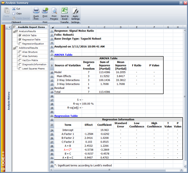
Other <math>S{{N}_{Ti}}\,\!</math> values can be obtained in a similar manner. The values are under the column Signal Noise Ratio in the data sheet shown above. As in the case of the location model, the analysis to fit the dispersion model can be carried out by treating the experiment as a single replicate of the <math>2^{3}\,\!</math> design. The results obtained from the DOE folio are shown in the figure below. | |||
[[Image:doe13_10.png|center|650px|Results for the dispersion model in the example.|link=]] | |||
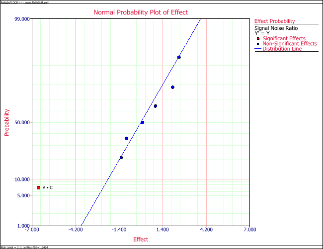
The normal probability plot of effects for this model (displayed next) shows that the interaction <math>AC\,\!</math> is the only significant effect for this model. | |||
[[Image:doe13_11.png|center|650px|Normal probability plot of effects for the dispersion model in the example.|link=]] | |||
Using the corresponding coefficient from the figure below, the dispersion model can be written as: | |||
::<math>S{{N}_{T}}=19.963-3.2869{{x}_{1}}{{x}_{3}}\,\!</math> | |||
where <math>{{x}_{3}}\,\!</math> is the variable representing factor <math>C\,\!</math>. | |||
'''Robust Parameter Design''' | '''Robust Parameter Design''' | ||
Following the analysis strategy mentioned in | Following the analysis strategy mentioned in [[Robust_Parameter_Design#Analysis_Strategy| Analysis Strategy]], for the nominal-the-best case, the dispersion model should be considered first. The equation for the model shows that to maximize <math>S{{N}_{T}}\,\!</math>, either one of the following options can be used: | ||
Then, considering the location model of | *<math>{{x}_{1}}=-1\,\!</math> and <math>{{x}_{3}}=+1\,\!</math> or | ||
*<math>{{x}_{1}}=+1\,\!</math> and <math>{{x}_{3}}=-1\,\!</math> | |||
Then, considering the location model of this example, to achieve a target response value as close to 7 as possible, the only significant effect for this model, <math>{{x}_{1}}\,\!</math>, should be set at the level of <math>-1\,\!</math>. Therefore, the first should be used for the dispersion model's settings. The final settings for the three factors, as a result of the robust parameter design, are: | |||
*Factor <math>A\,\!</math> is set at the low level | |||
*Factor <math>C\,\!</math> is set at the high level and | |||
*Factor <math>B\,\!</math>, which is not significant in any of the two models, can be set at the level that is most economical. | |||
With these settings the predicted pH value for the product is: | With these settings the predicted pH value for the product is: | ||
<math>\begin{align} | |||
::<math>\begin{align} | |||
\bar{y}= & 6.1781-0.7344{{x}_{1}} \\ | |||
= & 6.1781-0.7344(-1) \\ | |||
\end{align}</math> | = & 6.9125 | ||
\end{align}\,\!</math> | |||
The predicted signal to noise ratio is: | The predicted signal to noise ratio is: | ||
<math>\begin{align} | |||
::<math>\begin{align} | |||
S{{N}_{T}}= & 19.963-3.2869{{x}_{1}}{{x}_{3}} \\ | |||
= & 19.963-3.2869(-1)(1) \\ | |||
\end{align}</math> | = & 23.2499 | ||
\end{align}\,\!</math> | |||
To make the signal to noise ratio model hierarchical, | To make the signal to noise ratio model hierarchical, <math>{{x}_{1}}\,\!</math> and <math>{{x}_{3}},\,\!</math> have to be included in the model. Then, the predicted <math>SN\,\!</math> ratio is: | ||
::<math>\begin{align} | |||
S{{N}_{T}}= & 19.963-0.6292{{x}_{1}}+0.0515{{x}_{3}}-3.2869{{x}_{1}}{{x}_{3}} \\ | |||
= & 19.963-0.6292(-1)+0.0515(1)-3.2869(-1)(1) \\ | |||
= & 23.9306 | |||
\end{align}\,\!</math> | |||
==Limitations of Taguchi's Approach== | ==Limitations of Taguchi's Approach== | ||
Although Taguchi's approach towards robust parameter design introduced innovative techniques to improve quality, a few concerns regarding his philosophy have been raised. Some of these concerns relate to the signal to noise ratios defined to reduce variations in the response, and some others are related to the absence of the means to test for higher order control factor interactions when his orthogonal arrays are used as inner arrays for the design. For these reasons, other approaches to carry out robust parameter design have been suggested including response modeling and the use of <math>\ln s_{i}^{2}\,\!</math> in the place of the signal to noise ratios in the dispersion model. In response modeling, the noise factors are included in the model as additional factors, along with the other control factors. Details of these methods can be found in [[DOE_References|[Wu, 2000]]] and other theory books published on the subject. | |||
Although Taguchi's approach towards robust parameter design introduced innovative techniques to improve quality, a few concerns regarding his philosophy have been raised. Some of these concerns relate to the signal to noise ratios defined to reduce variations in the response, and some others are related to the absence of the means to test for higher | |||
Latest revision as of 17:03, 10 August 2017
In Response Surface Methods for Optimization, techniques used to optimize the response were discussed. Once an optimum value of the response has been achieved, the next goal of the experimenter should be to make the optimum response value insensitive to the noise factors so that a consistent performance is obtained at all times. For example, if the yield from a chemical process has been optimized at 95%, then this value of yield should be obtained regardless of the variation in factors such as the quality of reactants or fluctuations in humidity or other weather conditions. These factors are beyond the control of the operator. Therefore, the product or process should be such that it is not affected by minor fluctuations in these factors. The process of making a system insensitive to such factors is referred to as robust design. Robust design was pioneered by the Japanese industrialist Dr. Genichi Taguchi in the early 1980s. This chapter briefly discusses his approach.
Taguchi's Philosophy
Taguchi's philosophy is based on the fact that any decrease in the quality of a system leads to customer dissatisfaction. This occurs even if the departure in quality lies within the specified limits of the system and is considered acceptable to the customer. For example, consider the case of a laptop that develops a defect on its screen within the warranty period. Although the customer is able to get a warranty-replacement for the screen this might lead to a little dissatisfaction on the part of the customer. If the same laptop then develops a problem with its DVD drive, the customer might declare the laptop "useless," even if the problem occurs during the warranty period and the customer is able to get a free replacement. Therefore, to maintain a good reputation, the laptop manufacturer needs to produce laptops that offer the same quality to all customers consistently. This can only be done when the required quality is built into the laptops. Note how this approach differs from traditional quality control where it is considered sufficient to manufacture products within certain specifications and carry out pre-shipment quality control inspections (i.e., sampling inspections) to filter out products that fall out of specification.
Taguchi's philosophy requires that systems be designed in such a way that they are produced, not just within the specified limits, but right on target specifications or best values. Such a proactive approach is much more fruitful and efficient than the reactive approach of sampling inspections. The philosophy of Taguchi is summarized by his quality loss function (see the figure below). The function states that any deviation from the target value leads to a quadratic loss in quality or customer satisfaction. Mathematically, the function may be expressed as:
- [math]\displaystyle{ L=k{{(y-m)}^{2}}\,\! }[/math]
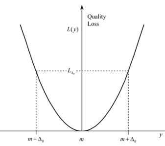
where [math]\displaystyle{ y\,\! }[/math] represents the performance parameter of the system, [math]\displaystyle{ m\,\! }[/math] represents the target or the nominal value of [math]\displaystyle{ y\,\! }[/math], [math]\displaystyle{ L\,\! }[/math] represents the quality loss and [math]\displaystyle{ k\,\! }[/math] is a constant.
Taguchi's approach to achieve a high quality system consists of three stages: system design, parameter design and tolerance design. System design refers to the stage when ideas for a new system are used to decide upon the combinations of factors to obtain a functional and economical design. Parameter design refers to the stage when factor settings are selected that make the system less sensitive to variations in the uncontrollable factors affecting the system. Therefore, if this stage is carried out successfully, the resulting system will have little variation and the resulting tolerances will be tight. Tolerance design refers to the final stage when tolerances are tightened around the best value. This stage increases cost and is only needed if the required quality is not achieved during parameter design. Thus, using parameter design, it is possible to achieve the desired quality without much increase in the cost. The tolerance design stage is discussed in detail next.
Robust Parameter Design
Taguchi divided the factors affecting any system into two categories: control factors and noise factors. Control factors are factors affecting a system that are easily set by the experimenter. For example, if in a chemical process the reaction time is found to be a factor affecting the yield, then this factor is a control factor since it can be easily manipulated and set by the experimenter. The experimenter will chose the setting of the reaction time that maximizes the yield. Noise factors are factors affecting a system that are difficult or impossible to control. For example, ambient temperature may also have an effect on the yield of a chemical process, but ambient temperature could be a noise factor if it is beyond the control of the experimenter. Thus, change in ambient temperature will lead to variations in the yield but such variations are undesirable.
Control and Noise Factor Interaction
In our example, since the experimenter does not have any control on the change in ambient temperature, he/she needs to find the setting of the reaction time at which there is minimal variation of yield due to change in ambient temperature. Note that this can only occur if there is an interaction between the reaction time (control factor) and ambient temperature (noise factor). If there is no such interaction, variation in yield due to changes in ambient temperature will always occur regardless of the setting of the reaction time. Therefore, to solve a robust parameter design problem, interaction between control and noise factors must exist. This fact is further explained by the figure shown next.
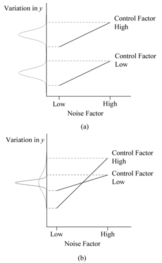
The figure shows the variation of the response (yield) for two levels of the noise factor (ambient temperature). The response values are plotted at two levels of the control factor (reaction time). Figure (a) shows the case where there is no interaction between the control and noise factors. It can be seen that, regardless of the settings of the control factor (low or high), the variation in the response remains the same (as is evident from the constant spread of the probability distribution of the response at the two levels of the control factor). Figure (b) shows the case where an interaction exists between the control and noise factors. The figure indicates that in the present case it is advantageous to have the control factor at the low setting, since at this setting there is not much variation in the response due to change in the noise factor (as is evident from the smaller spread of the probability distribution of the response at the low level of the control factor).
Inner and Outer Arrays
Taguchi studied the interaction between the control and noise factors using two experiment designs: the inner array and the outer array. The inner array is essentially any experiment design that is used to study the effect of the control factors on the response. Taguchi then used an outer array for the noise factors so that each run of the inner array was repeated for every treatment of the outer array. The resulting experiment design, that uses both inner and outer arrays, is referred to as a cross array.
Example
To illustrate Taguchi's use of the inner and outer arrays consider the case of a chemical process where the experimenter wants the product to be neither acidic nor basic (i.e., the pH of the product needs to be as close to 7 as possible). It is thought that the pH of the product depends on the concentration of the three reactants, [math]\displaystyle{ A\,\! }[/math], [math]\displaystyle{ B\,\! }[/math] and [math]\displaystyle{ C\,\! }[/math], used to obtain the product. There are three control factors here, namely the concentration of each of the three reactants. It has also been found that the pH of the product depends on the ambient temperature which varies naturally and cannot be controlled. Thus, there is one noise factor in this case - the ambient temperature. The experimenter chooses Taguchi's robust parameter design approach to investigate the settings of the control factors to make the product insensitive to changes in ambient temperature. It is decided to carry out a [math]\displaystyle{ 2^{3}\,\! }[/math] experiment to study the effect of the three control factors on the pH of the product. Therefore, the [math]\displaystyle{ 2^{3}\,\! }[/math] design is the inner array here. It is also decided to carry out the experiment at four levels of the ambient temperature by using a special enclosure where the surrounding temperature of the chemical process can be controlled. Therefore, the outer array consists of a single factor experiment with the factor at four levels. Note that, in order to carry out the robust parameter design approach, the noise factor should be such that it can be controlled in an experimental setting. The resulting setup of the robust parameter design experiment is shown in the following table.
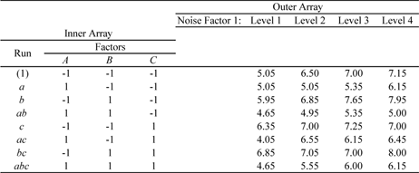
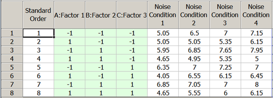
The experiment requires [math]\displaystyle{ 2^{3}\times 4=32\,\! }[/math] runs in all as each run of the inner array is repeated for every treatment of the outer array. The above table also shows the pH values obtained for the experiment. In a Weibull++ DOE folio, this design is set up by specifying the properties for the inner and outer arrays as shown in the following figure.
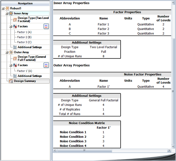
The resulting design is shown in the next figure.
Signal to Noise Ratios
Depending upon the objective of the robust parameter design, Taguchi defined three different statistics called signal to noise ratios. These ratios were defined as the means to measure the variation of the response with respect to the noise factors. Taguchi's approach essentially consists of two models: a location model and a dispersion model.
Location Model
The location model is the regression model for the mean value of the response at each treatment combination of the inner array. If [math]\displaystyle{ {{y}_{ij}}\,\! }[/math] ([math]\displaystyle{ j=1\,\! }[/math] [math]\displaystyle{ to\,\! }[/math] [math]\displaystyle{ m\,\! }[/math]) represents the [math]\displaystyle{ m\,\! }[/math] response values obtained at the [math]\displaystyle{ i\,\! }[/math]th treatment combination of the inner array (corresponding to the [math]\displaystyle{ m\,\! }[/math] levels of the noise factors), then the mean response at the [math]\displaystyle{ i\,\! }[/math]th level is:
- [math]\displaystyle{ {{\bar{y}}_{i}}=\frac{1}{m}\underset{j=1}{\overset{m}{\mathop \sum }}\,{{y}_{ij}}\,\! }[/math]
The location model is obtained by fitting a regression model to all [math]\displaystyle{ {{\bar{y}}_{i}}\,\! }[/math] values, by treating these values as the response at each of the [math]\displaystyle{ i\,\! }[/math]th treatments of the inner array. As an example, the location model for an inner array with two factors can be written as:
- [math]\displaystyle{ {{\bar{y}}_{i}}=\beta _{0}^{L}+\beta _{1}^{L}{{x}_{i1}}+\beta _{2}^{L}{{x}_{i2}}+\beta _{12}^{L}{{x}_{i1}}{{x}_{i2}}\,\! }[/math]
where:
- [math]\displaystyle{ \beta _{0}^{L}\,\! }[/math] is the intercept
- [math]\displaystyle{ \beta _{1}^{L}\,\! }[/math] is the coefficient for the first factor
- [math]\displaystyle{ \beta _{2}^{L}\,\! }[/math] is the coefficient for the second factor
- [math]\displaystyle{ \beta _{12}^{L}\,\! }[/math] is the coefficient for the interaction
- [math]\displaystyle{ {{x}_{1}}\,\! }[/math] and [math]\displaystyle{ {{x}_{2}}\,\! }[/math] are respectively the variables for the two factors
The objective of using the location model is to bring the response to its goal regardless of whether this is a target value, maximum value or minimum value. This is done by identifying significant effects and then using the least square estimates of the corresponding coefficients, [math]\displaystyle{ {{\beta }^{L}}\,\! }[/math]s, to fit the location model. The fitted model is used to decide the settings of the variables that bring the response to the goal.
Dispersion Model
The dispersion model measures the variation of the response due to the noise factors. The standard deviation of the response values at each treatment combination, [math]\displaystyle{ {{s}_{i}}\,\! }[/math], is used. Usually, the standard deviation is used as a log function of [math]\displaystyle{ s_{i}^{2}\,\! }[/math] because [math]\displaystyle{ \ln s_{i}^{2}\,\! }[/math] are approximately normally distributed. These values can be calculated as follows:
- [math]\displaystyle{ \ln s_{i}^{2}=\ln (\frac{\mathop{}_{j=1}^{m}{{({{y}_{ij}}-{{{\bar{y}}}_{i}})}^{2}}}{m-1})\,\! }[/math]
Thus, the dispersion model consists of using [math]\displaystyle{ \ln s_{i}^{2}\,\! }[/math] as the response and investigating what treatment of the control factors results in the minimum variation of the response. Clearly, the objective of using the dispersion model is to minimize variation in the response. Instead of using standard deviations directly, Taguchi defined three signal to noise ratios (abbreviated [math]\displaystyle{ SN\,\! }[/math]) based on the objective function for the response. If the response is to be maximized, the [math]\displaystyle{ SN\,\! }[/math] ratio is defined as follows:
- [math]\displaystyle{ S{{N}_{L}}=-10{{\log }_{10}}(\frac{1}{m}\underset{j=1}{\overset{m}{\mathop \sum }}\,\frac{1}{y_{ij}^{2}})\,\! }[/math]
The previous ratio is referred to as the larger-the-better ratio and is defined to decrease variability when maximizing the response.
When the response is to be minimized, the [math]\displaystyle{ SN\,\! }[/math] ratio is defined as:
- [math]\displaystyle{ S{{N}_{S}}=-10{{\log }_{10}}(\frac{1}{m}\underset{j=1}{\overset{m}{\mathop \sum }}\,y_{ij}^{2})\,\! }[/math]
This ratio is referred to as the smaller-the-better ratio and is defined to decrease variability when minimizing the response.
If the objective for the response is to achieve a target or nominal value, then the [math]\displaystyle{ SN\,\! }[/math] ratio is defined as follows:
- [math]\displaystyle{ S{{N}_{T}}=10{{\log }_{10}}(\frac{\bar{y}_{i}^{2}}{s_{i}^{2}})\,\! }[/math]
This ratio is referred to as the nominal-the-best ratio and is defined to decrease variability around a target response value.
The dispersion model for any of the three signal to noise ratios can be written as follows for an inner array with two factors:
- [math]\displaystyle{ SN=\beta _{0}^{D}+\beta _{1}^{D}{{x}_{1}}+\beta _{2}^{D}{{x}_{2}}+\beta _{12}^{D}{{x}_{1}}{{x}_{2}}\,\! }[/math]
where:
- [math]\displaystyle{ \beta _{0}^{D}\,\! }[/math] is the intercept
- [math]\displaystyle{ \beta _{1}^{D}\,\! }[/math] is the coefficient for the first factor
- [math]\displaystyle{ \beta _{2}^{D}\,\! }[/math] is the coefficient for the second factor
- [math]\displaystyle{ \beta _{12}^{D}\,\! }[/math] is the coefficient for the interaction
- [math]\displaystyle{ {{x}_{1}}\,\! }[/math] and [math]\displaystyle{ {{x}_{2}}\,\! }[/math] are respectively the variables for the two factors
The dispersion model is fit by identifying significant effects and then using the least square estimates of the coefficients [math]\displaystyle{ {{\beta }^{D}}\,\! }[/math]s. Once the fitted dispersion model is known, settings for the control factors are found that result in the maximum value of [math]\displaystyle{ SN\,\! }[/math], thereby minimizing the response variation.
Analysis Strategy
The location and dispersion regression models are usually obtained by using graphical techniques to identify significant effects. This is because the responses used in the two models are such that only one response value is obtained for each treatment of the inner array. Therefore, the experiment design in the case of the two models is an unreplicated design.
Once the location and dispersion models have been obtained by identification of the significant effects, the following analysis strategy [Wu, 2000] may be used:
- To obtain the best settings of the factors for larger-the-better and smaller-the-better cases:
- The experimenter must first select the settings of the significant control factors in the location model to either maximize or minimize the response.
- Then the experimenter must choose the settings of those significant control factors in the dispersion model, that are not significant in the location model, to maximize the [math]\displaystyle{ SN\,\! }[/math] ratio.
- For nominal-the-best cases:
- The experimenter must first select the settings of the significant control factors in the dispersion model to maximize the [math]\displaystyle{ SN\,\! }[/math] ratio.
- Then the experimenter must choose the levels of the significant control factors in the location model to bring the response on target. At times, the same control factor(s) may show up as significant in both the location and dispersion models. In these cases, the experimenter must use his judgement to obtain the best settings of the control factors based upon the two models.
Factors that do not show up as significant in both the models should be set at levels that result in the greatest economy. Generally, a follow-up experiment is usually carried out with the best settings to verify that the system functions as desired.
Example
This example illustrates the procedure to obtain the location and dispersion models for the experiment in the previous example.
Location Model
The response values used in the location model can be calculated using the first equation given in Location Model. As an example, the response value for the third treatment is:
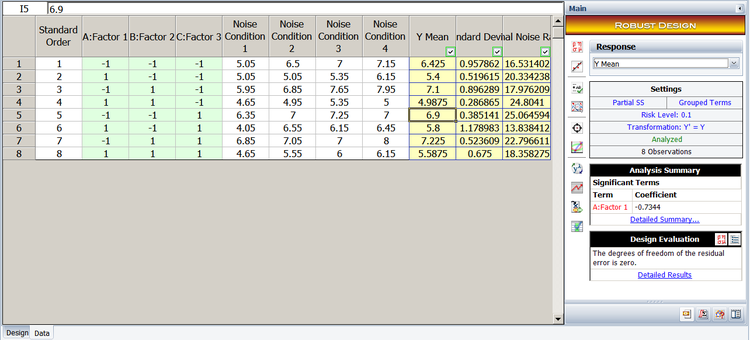
- [math]\displaystyle{ \begin{align} {{{\bar{y}}}_{3}}= & \frac{1}{m}\underset{j=1}{\overset{m}{\mathop \sum }}\,{{y}_{3j}} \\ = & \frac{1}{4}({{y}_{31}}+{{y}_{32}}+{{y}_{33}}+{{y}_{34}}) \\ = & \frac{1}{4}(5.95+6.85+7.65+7.95) \\ = & 7.1 \end{align}\,\! }[/math]
Response values for the remaining seven treatments can be calculated in a similar manner. These values are shown next under the Y Mean column.
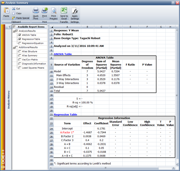
Once the response values for all the treatments are known, the analysis to fit the location model can be carried out by treating the experiment as a single replicate of the [math]\displaystyle{ 2^{3}\,\! }[/math] design. The results obtained from the DOE folio are shown in the figure below.
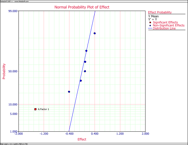
The normal probability plot of effects for this model shows that only the main effect of factor [math]\displaystyle{ A\,\! }[/math] is significant for the location model (see the figure below).
Using the corresponding coefficient from the figure below, the location model can be written as:
- [math]\displaystyle{ \bar{y}=6.1781-0.7344{{x}_{1}}\,\! }[/math]
where [math]\displaystyle{ {{x}_{1}}\,\! }[/math] is the variable representing factor [math]\displaystyle{ A\,\! }[/math].
Dispersion Model
For the dispersion model, the applicable signal to noise ratio is given by the equation for the nominal-the-best ratio:
- [math]\displaystyle{ S{{N}_{Ti}}=-10{{\log }_{10}}(\frac{\bar{y}_{i}^{2}}{s_{i}^{2}})\,\! }[/math]
The response values for the dispersion model can now be calculated. As an example, the response value for the third treatment is:
- [math]\displaystyle{ \begin{align} S{{N}_{T3}}= & -10{{\log }_{10}}(\frac{\bar{y}_{3}^{2}}{s_{1}^{2}}) \\ = & -10{{\log }_{10}}(\frac{\bar{y}_{3}^{2}}{\tfrac{1}{(4-1)}\mathop{}_{j=1}^{4}{{({{y}_{3j}}-{{{\bar{y}}}_{3}})}^{2}}}) \\ = & -10{{\log }_{10}}(\frac{{{7.1}^{2}}}{{{0.8963}^{2}}}) \\ = & 17.9762 \end{align}\,\! }[/math]
Other [math]\displaystyle{ S{{N}_{Ti}}\,\! }[/math] values can be obtained in a similar manner. The values are under the column Signal Noise Ratio in the data sheet shown above. As in the case of the location model, the analysis to fit the dispersion model can be carried out by treating the experiment as a single replicate of the [math]\displaystyle{ 2^{3}\,\! }[/math] design. The results obtained from the DOE folio are shown in the figure below.
The normal probability plot of effects for this model (displayed next) shows that the interaction [math]\displaystyle{ AC\,\! }[/math] is the only significant effect for this model.
Using the corresponding coefficient from the figure below, the dispersion model can be written as:
- [math]\displaystyle{ S{{N}_{T}}=19.963-3.2869{{x}_{1}}{{x}_{3}}\,\! }[/math]
where [math]\displaystyle{ {{x}_{3}}\,\! }[/math] is the variable representing factor [math]\displaystyle{ C\,\! }[/math].
Robust Parameter Design
Following the analysis strategy mentioned in Analysis Strategy, for the nominal-the-best case, the dispersion model should be considered first. The equation for the model shows that to maximize [math]\displaystyle{ S{{N}_{T}}\,\! }[/math], either one of the following options can be used:
- [math]\displaystyle{ {{x}_{1}}=-1\,\! }[/math] and [math]\displaystyle{ {{x}_{3}}=+1\,\! }[/math] or
- [math]\displaystyle{ {{x}_{1}}=+1\,\! }[/math] and [math]\displaystyle{ {{x}_{3}}=-1\,\! }[/math]
Then, considering the location model of this example, to achieve a target response value as close to 7 as possible, the only significant effect for this model, [math]\displaystyle{ {{x}_{1}}\,\! }[/math], should be set at the level of [math]\displaystyle{ -1\,\! }[/math]. Therefore, the first should be used for the dispersion model's settings. The final settings for the three factors, as a result of the robust parameter design, are:
- Factor [math]\displaystyle{ A\,\! }[/math] is set at the low level
- Factor [math]\displaystyle{ C\,\! }[/math] is set at the high level and
- Factor [math]\displaystyle{ B\,\! }[/math], which is not significant in any of the two models, can be set at the level that is most economical.
With these settings the predicted pH value for the product is:
- [math]\displaystyle{ \begin{align} \bar{y}= & 6.1781-0.7344{{x}_{1}} \\ = & 6.1781-0.7344(-1) \\ = & 6.9125 \end{align}\,\! }[/math]
The predicted signal to noise ratio is:
- [math]\displaystyle{ \begin{align} S{{N}_{T}}= & 19.963-3.2869{{x}_{1}}{{x}_{3}} \\ = & 19.963-3.2869(-1)(1) \\ = & 23.2499 \end{align}\,\! }[/math]
To make the signal to noise ratio model hierarchical, [math]\displaystyle{ {{x}_{1}}\,\! }[/math] and [math]\displaystyle{ {{x}_{3}},\,\! }[/math] have to be included in the model. Then, the predicted [math]\displaystyle{ SN\,\! }[/math] ratio is:
- [math]\displaystyle{ \begin{align} S{{N}_{T}}= & 19.963-0.6292{{x}_{1}}+0.0515{{x}_{3}}-3.2869{{x}_{1}}{{x}_{3}} \\ = & 19.963-0.6292(-1)+0.0515(1)-3.2869(-1)(1) \\ = & 23.9306 \end{align}\,\! }[/math]
Limitations of Taguchi's Approach
Although Taguchi's approach towards robust parameter design introduced innovative techniques to improve quality, a few concerns regarding his philosophy have been raised. Some of these concerns relate to the signal to noise ratios defined to reduce variations in the response, and some others are related to the absence of the means to test for higher order control factor interactions when his orthogonal arrays are used as inner arrays for the design. For these reasons, other approaches to carry out robust parameter design have been suggested including response modeling and the use of [math]\displaystyle{ \ln s_{i}^{2}\,\! }[/math] in the place of the signal to noise ratios in the dispersion model. In response modeling, the noise factors are included in the model as additional factors, along with the other control factors. Details of these methods can be found in [Wu, 2000] and other theory books published on the subject.
