Degradation Data Analysis with a Power Regression Model: Difference between revisions
Jump to navigation
Jump to search
Kate Racaza (talk | contribs) (Created page with '{{Reference Example}} This example compares the results for a degradation analysis with a power regression model. {{Reference_Example_Heading1}} The data set is from Example …') |
Kate Racaza (talk | contribs) No edit summary |
||
| (One intermediate revision by the same user not shown) | |||
| Line 1: | Line 1: | ||
{{Reference Example}} | {{Reference Example}} | ||
This example | This example validates the results for a degradation analysis with a power regression model in Weibull++ degradation folios. | ||
| Line 98: | Line 98: | ||
In the book, the following equation is used: <math>ln(y) = \beta_{1} + \beta_{2} ln(t)\,\!</math>. It in fact is a power equation <math>y = bt^{a}\,\!</math> with <math>ln(b) = \beta_{1}\,\!</math> and <math>a = \beta_{2}\,\!</math>. This degradation equation is used for each test unit to predict the pseudo failure time, and then a lognormal distribution is used to model the pseudo failure times. The results are: | In the book, the following equation is used: <math>ln(y) = \beta_{1} + \beta_{2} ln(t)\,\!</math>. It in fact is a power equation <math>y = bt^{a}\,\!</math> with <math>ln(b) = \beta_{1}\,\!</math> and <math>a = \beta_{2}\,\!</math>. This degradation equation is used for each test unit to predict the pseudo failure time, and then a lognormal distribution is used to model the pseudo failure times. The results are: | ||
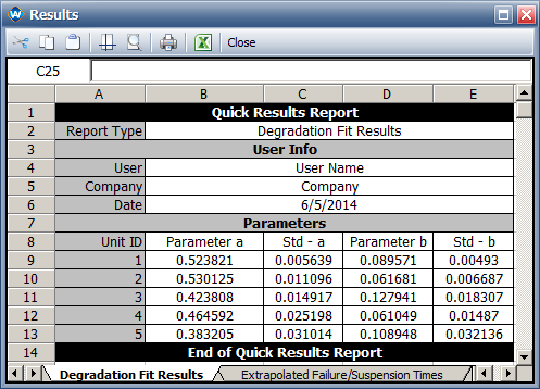
* | * The parameters of the power regression model for each unit are: | ||
:* For unit 1 <math>\beta_{1}\,\!</math> = -2.413 , <math>\beta_{2}\,\!</math> = 0.524 | :* For unit 1: <math>\beta_{1}\,\!</math> = -2.413 , <math>\beta_{2}\,\!</math> = 0.524 | ||
:* For unit 2 <math>\beta_{1}\,\!</math> = -2.735 , <math>\beta_{2}\,\!</math> = 0.525 | :* For unit 2: <math>\beta_{1}\,\!</math> = -2.735 , <math>\beta_{2}\,\!</math> = 0.525 | ||
:* For unit 3 <math>\beta_{1}\,\!</math> = -2.056 , <math>\beta_{2}\,\!</math> = 0.424 | :* For unit 3: <math>\beta_{1}\,\!</math> = -2.056 , <math>\beta_{2}\,\!</math> = 0.424 | ||
:* For unit 4 <math>\beta_{1}\,\!</math> = -2.796 , <math>\beta_{2}\,\!</math> = 0.465 | :* For unit 4: <math>\beta_{1}\,\!</math> = -2.796 , <math>\beta_{2}\,\!</math> = 0.465 | ||
:* For unit 5 <math>\beta_{1}\,\!</math> = -2.217 , <math>\beta_{2}\,\!</math> = 0.383 | :* For unit 5: <math>\beta_{1}\,\!</math> = -2.217 , <math>\beta_{2}\,\!</math> = 0.383 | ||
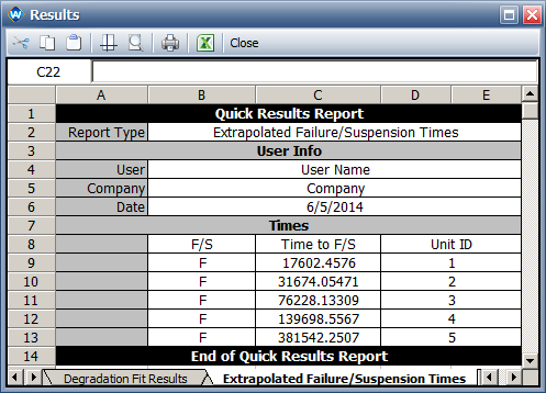
* The predicted pseudo failure times: 17,553; 31,816; 75,809; 138,229. | * The predicted pseudo failure times are: 17,553; 31,816; 75,809; 138,229. | ||
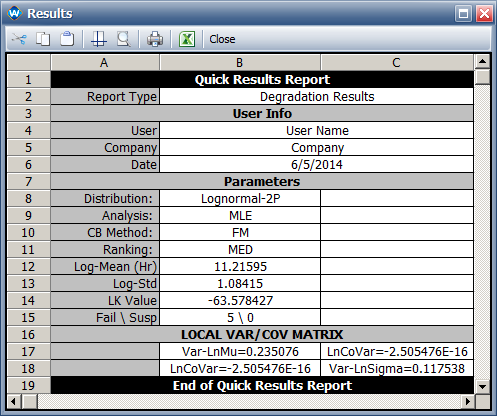
* The fitted lognormal distribution: Ln-Mean = 11.214, Ln-Std = 1.085. | * The parameters of the fitted lognormal distribution are: Ln-Mean = 11.214, Ln-Std = 1.085. | ||
{{Reference_Example_Heading4}} | {{Reference_Example_Heading4}} | ||
* | * The following picture shows the parameters of the power regression model for each unit. | ||
[[Image:DA_pwr_model.png|center]] | [[Image:DA_pwr_model.png|center]] | ||
* The predicted pseudo failure times | * The predicted pseudo failure times are shown next. | ||
[[Image:DA_extrapolated.png|center]] | [[Image:DA_extrapolated.png|center]] | ||
* The fitted lognormal distribution | * The next picture shows the parameters of the fitted lognormal distribution. | ||
[[Image:DA_log_model.png|center]] | [[Image:DA_log_model.png|center]] | ||
Latest revision as of 16:22, 28 September 2015
New format available! This reference is now available in a new format that offers faster page load, improved display for calculations and images and more targeted search.
As of January 2024, this Reliawiki page will not continue to be updated. Please update all links and bookmarks to the latest references at Weibull examples and Weibull reference examples.


