Use of Regression to Calculate Sum of Squares: Difference between revisions
Chris Kahn (talk | contribs) No edit summary |
Lisa Hacker (talk | contribs) No edit summary |
||
| (8 intermediate revisions by 2 users not shown) | |||
| Line 1: | Line 1: | ||
{{Template: | {{Template:Doebook|Appendix B|Use of Regression to Calculate Sum of Squares}} | ||
This appendix explains the reason behind the use of regression in | This appendix explains the reason behind the use of regression in Weibull++ DOE folios in all calculations related to the sum of squares. A number of textbooks present the method of direct summation to calculate the sum of squares. But this method is only applicable for balanced designs and may give incorrect results for unbalanced designs. For example, the sum of squares for factor <math>A\,\!</math> in a balanced factorial experiment with two factors, <math>A\,\!</math> and <math>B\,\!</math>, is given as follows: | ||
| Line 37: | Line 37: | ||
which is obviously incorrect since the sum of squares cannot be negative. For a detailed discussion on this refer to [[ | which is obviously incorrect since the sum of squares cannot be negative. For a detailed discussion on this refer to [[DOE References|Searle(1997, 1971)]]. | ||
[[Image:doet6.6.png | [[Image:doet6.6.png|center|325px|Example of an unbalanced design.|link=]] | ||
| Line 77: | Line 77: | ||
This is the value that is calculated by DOE | This is the value that is calculated by the DOE folio (see the first figure below, for the experiment design and the second figure below for the analysis). | ||
[[Image: | [[Image:doe6_15.png|center|600px|Unbalanced experimental design for the data in the last table.|link=]] | ||
[[Image: | [[Image:doe6_16_1.png|center|471px|Analysis for the unbalanced data in the last table.|link=]] | ||
Latest revision as of 19:07, 15 September 2023
This appendix explains the reason behind the use of regression in Weibull++ DOE folios in all calculations related to the sum of squares. A number of textbooks present the method of direct summation to calculate the sum of squares. But this method is only applicable for balanced designs and may give incorrect results for unbalanced designs. For example, the sum of squares for factor [math]\displaystyle{ A\,\! }[/math] in a balanced factorial experiment with two factors, [math]\displaystyle{ A\,\! }[/math] and [math]\displaystyle{ B\,\! }[/math], is given as follows:
- [math]\displaystyle{ \begin{align} & S{{S}_{A}}= & \underset{i=1}{\overset{{{n}_{a}}}{\mathop{\sum }}}\,{{n}_{b}}n{{({{{\bar{y}}}_{i..}}-{{{\bar{y}}}_{...}})}^{2}} \\ & = & \underset{i=1}{\overset{{{n}_{a}}}{\mathop{\sum }}}\,\frac{y_{i..}^{2}}{{{n}_{b}}n}-\frac{y_{...}^{2}}{{{n}_{a}}{{n}_{b}}n} \end{align}\,\! }[/math]
where [math]\displaystyle{ {{n}_{a}}\,\! }[/math] represents the levels of factor [math]\displaystyle{ A\,\! }[/math], [math]\displaystyle{ {{n}_{b}}\,\! }[/math] represents the levels of factor [math]\displaystyle{ B\,\! }[/math], and [math]\displaystyle{ n\,\! }[/math] represents the number of samples for each combination of [math]\displaystyle{ A\,\! }[/math] and [math]\displaystyle{ B\,\! }[/math]. The term [math]\displaystyle{ {{\bar{y}}_{i..}}\,\! }[/math] is the mean value for the [math]\displaystyle{ i\,\! }[/math]th level of factor [math]\displaystyle{ A\,\! }[/math], [math]\displaystyle{ {{y}_{i..}}\,\! }[/math] is the sum of all observations at the [math]\displaystyle{ i\,\! }[/math]th level of factor [math]\displaystyle{ A\,\! }[/math] and [math]\displaystyle{ {{y}_{...}}\,\! }[/math] is the sum of all observations.
The analogous term to calculate [math]\displaystyle{ S{{S}_{A}}\,\! }[/math] in the case of an unbalanced design is given as:
- [math]\displaystyle{ S{{S}_{A}}=\underset{i=1}{\overset{{{n}_{a}}}{\mathop{\sum }}}\,\frac{y_{i..}^{2}}{{{n}_{i.}}}-\frac{y_{...}^{2}}{{{n}_{..}}}\,\! }[/math]
where [math]\displaystyle{ {{n}_{i.}}\,\! }[/math] is the number of observations at the [math]\displaystyle{ i\,\! }[/math]th level of factor [math]\displaystyle{ A\,\! }[/math] and [math]\displaystyle{ {{n}_{..}}\,\! }[/math] is the total number of observations. Similarly, to calculate the sum of squares for factor [math]\displaystyle{ B\,\! }[/math] and interaction [math]\displaystyle{ AB\,\! }[/math], the formulas are given as:
- [math]\displaystyle{ \begin{align} & S{{S}_{B}}= & \underset{j=1}{\overset{{{n}_{b}}}{\mathop{\sum }}}\,\frac{y_{.j.}^{2}}{{{n}_{.j}}}-\frac{y_{...}^{2}}{{{n}_{..}}} \\ & S{{S}_{AB}}= & \underset{i=1}{\overset{{{n}_{a}}}{\mathop{\sum }}}\,\underset{j=1}{\overset{{{n}_{b}}}{\mathop{\sum }}}\,\frac{y_{ij.}^{2}}{{{n}_{ij}}}-\underset{i=1}{\overset{{{n}_{a}}}{\mathop{\sum }}}\,\frac{y_{i..}^{2}}{{{n}_{i.}}}-\underset{j=1}{\overset{{{n}_{b}}}{\mathop{\sum }}}\,\frac{y_{.j.}^{2}}{{{n}_{.j}}}+\frac{y_{...}^{2}}{{{n}_{..}}} \end{align}\,\! }[/math]
Applying these relations to the unbalanced data of the last table, the sum of squares for the interaction [math]\displaystyle{ AB\,\! }[/math] is:
- [math]\displaystyle{ \begin{align} & S{{S}_{AB}}= & \underset{i=1}{\overset{{{n}_{a}}}{\mathop{\sum }}}\,\underset{j=1}{\overset{{{n}_{b}}}{\mathop{\sum }}}\,\frac{y_{ij.}^{2}}{{{n}_{ij}}}-\underset{i=1}{\overset{{{n}_{a}}}{\mathop{\sum }}}\,\frac{y_{i..}^{2}}{{{n}_{i.}}}-\underset{j=1}{\overset{{{n}_{b}}}{\mathop{\sum }}}\,\frac{y_{.j.}^{2}}{{{n}_{.j}}}+\frac{y_{...}^{2}}{{{n}_{..}}} \\ & = & \left( {{6}^{2}}+{{4}^{2}}+\frac{{{(42+6)}^{2}}}{2}+{{12}^{2}} \right)-\left( \frac{{{10}^{2}}}{2}+\frac{{{60}^{2}}}{3} \right) \\ & & -\left( \frac{{{54}^{2}}}{3}+\frac{{{16}^{2}}}{2} \right)+\frac{{{70}^{2}}}{5} \\ & = & -22 \end{align}\,\! }[/math]
which is obviously incorrect since the sum of squares cannot be negative. For a detailed discussion on this refer to Searle(1997, 1971).

The correct sum of squares can be calculated as shown next. The [math]\displaystyle{ y\,\! }[/math] and [math]\displaystyle{ X\,\! }[/math] matrices for the design of the last table can be written as:
Then the sum of squares for the interaction [math]\displaystyle{ AB\,\! }[/math] can be calculated as:
- [math]\displaystyle{ S{{S}_{AB}}={{y}^{\prime }}[H-(1/5)J]y-{{y}^{\prime }}[{{H}_{\tilde{\ }AB}}-(1/5)J]y\,\! }[/math]
where [math]\displaystyle{ H\,\! }[/math] is the hat matrix and [math]\displaystyle{ J\,\! }[/math] is the matrix of ones. The matrix [math]\displaystyle{ {{H}_{\tilde{\ }AB}}\,\! }[/math] can be calculated using [math]\displaystyle{ {{H}_{\tilde{\ }AB}}={{X}_{\tilde{\ }AB}}{{(X_{\tilde{\ }AB}^{\prime }{{X}_{\tilde{\ }AB}})}^{-1}}X_{\tilde{\ }AB}^{\prime }\,\! }[/math] where [math]\displaystyle{ {{X}_{\tilde{\ }AB}}\,\! }[/math] is the design matrix, [math]\displaystyle{ X\,\! }[/math], excluding the last column that represents the interaction effect [math]\displaystyle{ AB\,\! }[/math]. Thus, the sum of squares for the interaction [math]\displaystyle{ AB\,\! }[/math] is:
- [math]\displaystyle{ \begin{align} & S{{S}_{AB}}= & {{y}^{\prime }}[H-(1/5)J]y-{{y}^{\prime }}[{{H}_{\tilde{\ }AB}}-(1/5)J]y \\ & = & 368-339.4286 \\ & = & 28.5714 \end{align}\,\! }[/math]
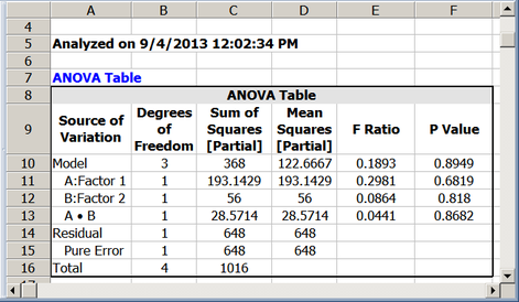
This is the value that is calculated by the DOE folio (see the first figure below, for the experiment design and the second figure below for the analysis).


