Parametric Binomial Example - Demonstrate Reliability: Difference between revisions
Chris Kahn (talk | contribs) No edit summary |
Lisa Hacker (talk | contribs) No edit summary |
||
| (4 intermediate revisions by 3 users not shown) | |||
| Line 1: | Line 1: | ||
<noinclude>{{Banner Weibull Examples}} | <noinclude>{{Banner Weibull Examples}} | ||
''This example appears in the [ | ''This example appears in the [https://help.reliasoft.com/reference/life_data_analysis Life data analysis reference]''. | ||
</noinclude> | </noinclude> | ||
In this example, we will use the parametric binomial method to design a test to demonstrate a reliability of 90% at <math>{{t}_{DEMO}}=100</math> hours with 95% confidence if no failure occur during the test. We will assume a Weibull distribution with a shape parameter | In this example, we will use the parametric binomial method to design a test to demonstrate a reliability of 90% at <math>{{t}_{DEMO}}=100\,\!</math> hours with a 95% confidence if no failure occur during the test. We will assume a Weibull distribution with a shape parameter <math>\beta =1.5\,\!</math>. | ||
'''Determining Units for Available Test Time''' | '''Determining Units for Available Test Time''' | ||
In the above scenario, we know that we have the testing facilities available for | In the above scenario, we know that we have the testing facilities available for <math>t=48\,\!</math> hours. We must now determine the number of units to test for this amount of time with no failures in order to have demonstrated our reliability goal. | ||
The first step is to determine the Weibull scale parameter, | The first step is to determine the Weibull scale parameter, <math>\eta \,\!</math>. The Weibull reliability equation is: | ||
::<math>R={{e}^{-{{(t/\eta )}^{\beta }}}}</math> | ::<math>R={{e}^{-{{(t/\eta )}^{\beta }}}}\,\!</math> | ||
This can be rewritten as: | This can be rewritten as: | ||
::<math>\eta =\frac{{{t}_{DEMO}}}{{{(-\text{ln}({{R}_{DEMO}}))}^{\tfrac{1}{\beta }}}}</math> | ::<math>\eta =\frac{{{t}_{DEMO}}}{{{(-\text{ln}({{R}_{DEMO}}))}^{\tfrac{1}{\beta }}}}\,\!</math> | ||
Since we know the values of | Since we know the values of <math>{{t}_{DEMO}}\,\!</math>, <math>{{R}_{DEMO}}\,\!</math> and <math>\beta \,\!</math>, we can substitute these in the equation and solve for <math>\eta \,\!</math>: | ||
::<math>\eta =\frac{100}{{{(-\text{ln}(0.9))}^{\tfrac{1}{1.5}}}}=448.3</math> | ::<math>\eta =\frac{100}{{{(-\text{ln}(0.9))}^{\tfrac{1}{1.5}}}}=448.3\,\!</math> | ||
Next, the value of <math>{{R}_{TEST}}</math> is calculated by: | Next, the value of <math>{{R}_{TEST}}\,\!</math> is calculated by: | ||
::<math>{{R}_{TEST}}={{e}^{-{{({{t}_{TEST}}/\eta )}^{\beta }}}}={{e}^{-{{(48/448.3)}^{1.5}}}}=0.966=96.6%</math> | ::<math>{{R}_{TEST}}={{e}^{-{{({{t}_{TEST}}/\eta )}^{\beta }}}}={{e}^{-{{(48/448.3)}^{1.5}}}}=0.966=96.6%\,\!</math> | ||
The last step is to substitute the appropriate values into the cumulative binomial equation, which for the Weibull distribution appears as: | The last step is to substitute the appropriate values into the cumulative binomial equation, which for the Weibull distribution appears as: | ||
::<math>1-CL=\underset{i=0}{\overset{f}{\mathop \sum }}\,\frac{n!}{i!\cdot (n-i)!}\cdot {{(1-{{e}^{-{{({{t}_{TEST}}/\eta )}^{\beta }}}})}^{i}}\cdot {{({{e}^{-{{({{t}_{TEST}}/\eta )}^{\beta }}}})}^{(n-i)}}</math> | ::<math>1-CL=\underset{i=0}{\overset{f}{\mathop \sum }}\,\frac{n!}{i!\cdot (n-i)!}\cdot {{(1-{{e}^{-{{({{t}_{TEST}}/\eta )}^{\beta }}}})}^{i}}\cdot {{({{e}^{-{{({{t}_{TEST}}/\eta )}^{\beta }}}})}^{(n-i)}}\,\!</math> | ||
The values of | The values of <math>CL\,\!</math>, <math>{{t}_{TEST}}\,\!</math>, <math>\beta \,\!</math>, <math>f\,\!</math> and <math>\eta \,\!</math> have already been calculated or specified, so it merely remains to solve the equation for <math>n\,\!</math>. This value is <math>n=85.4994\,\!</math>, or <math>n=86\,\!</math> units, since the fractional value must be rounded up to the next integer value. This example solved in Weibull++ is shown next. | ||
[[Image:RDT Weibull Demonstrate Reliability Test Time.png|center|800px]] | |||
'''Determining Time for Available Units''' | '''Determining Time for Available Units''' | ||
In this case, we will assume that we have 20 units to test, | In this case, we will assume that we have 20 units to test, <math>n=20\,\!</math>, and must determine the test time, <math>{{t}_{TEST}}\,\!</math>. We have already determined the value of the scale parameter, <math>\eta \,\!</math>, in the previous example. Since we know the values of <math>n\,\!</math>, <math>CL\,\!</math>, <math>f\,\!</math>, <math>\eta \,\!</math> and <math>\beta \,\!</math>, it remains to solve the binomial equation with the Weibull distribution for <math>{{t}_{TEST}}\,\!</math>. This value is <math>{{t}_{TEST}}=126.4339\,\!</math> hours. This example solved in Weibull++ is shown next. | ||
<br> | <br> | ||
[[Image:RDT Weibull Demonstrate Reliability | [[Image:RDT Weibull Demonstrate Reliability Samples.png|center|800px]] | ||
Latest revision as of 18:30, 18 September 2023
New format available! This reference is now available in a new format that offers faster page load, improved display for calculations and images and more targeted search.
As of January 2024, this Reliawiki page will not continue to be updated. Please update all links and bookmarks to the latest references at Weibull examples and Weibull reference examples.
This example appears in the Life data analysis reference.
In this example, we will use the parametric binomial method to design a test to demonstrate a reliability of 90% at [math]\displaystyle{ {{t}_{DEMO}}=100\,\! }[/math] hours with a 95% confidence if no failure occur during the test. We will assume a Weibull distribution with a shape parameter [math]\displaystyle{ \beta =1.5\,\! }[/math].
Determining Units for Available Test Time
In the above scenario, we know that we have the testing facilities available for [math]\displaystyle{ t=48\,\! }[/math] hours. We must now determine the number of units to test for this amount of time with no failures in order to have demonstrated our reliability goal. The first step is to determine the Weibull scale parameter, [math]\displaystyle{ \eta \,\! }[/math]. The Weibull reliability equation is:
- [math]\displaystyle{ R={{e}^{-{{(t/\eta )}^{\beta }}}}\,\! }[/math]
This can be rewritten as:
- [math]\displaystyle{ \eta =\frac{{{t}_{DEMO}}}{{{(-\text{ln}({{R}_{DEMO}}))}^{\tfrac{1}{\beta }}}}\,\! }[/math]
Since we know the values of [math]\displaystyle{ {{t}_{DEMO}}\,\! }[/math], [math]\displaystyle{ {{R}_{DEMO}}\,\! }[/math] and [math]\displaystyle{ \beta \,\! }[/math], we can substitute these in the equation and solve for [math]\displaystyle{ \eta \,\! }[/math]:
- [math]\displaystyle{ \eta =\frac{100}{{{(-\text{ln}(0.9))}^{\tfrac{1}{1.5}}}}=448.3\,\! }[/math]
Next, the value of [math]\displaystyle{ {{R}_{TEST}}\,\! }[/math] is calculated by:
- [math]\displaystyle{ {{R}_{TEST}}={{e}^{-{{({{t}_{TEST}}/\eta )}^{\beta }}}}={{e}^{-{{(48/448.3)}^{1.5}}}}=0.966=96.6%\,\! }[/math]
The last step is to substitute the appropriate values into the cumulative binomial equation, which for the Weibull distribution appears as:
- [math]\displaystyle{ 1-CL=\underset{i=0}{\overset{f}{\mathop \sum }}\,\frac{n!}{i!\cdot (n-i)!}\cdot {{(1-{{e}^{-{{({{t}_{TEST}}/\eta )}^{\beta }}}})}^{i}}\cdot {{({{e}^{-{{({{t}_{TEST}}/\eta )}^{\beta }}}})}^{(n-i)}}\,\! }[/math]
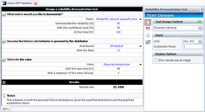
The values of [math]\displaystyle{ CL\,\! }[/math], [math]\displaystyle{ {{t}_{TEST}}\,\! }[/math], [math]\displaystyle{ \beta \,\! }[/math], [math]\displaystyle{ f\,\! }[/math] and [math]\displaystyle{ \eta \,\! }[/math] have already been calculated or specified, so it merely remains to solve the equation for [math]\displaystyle{ n\,\! }[/math]. This value is [math]\displaystyle{ n=85.4994\,\! }[/math], or [math]\displaystyle{ n=86\,\! }[/math] units, since the fractional value must be rounded up to the next integer value. This example solved in Weibull++ is shown next.
Determining Time for Available Units
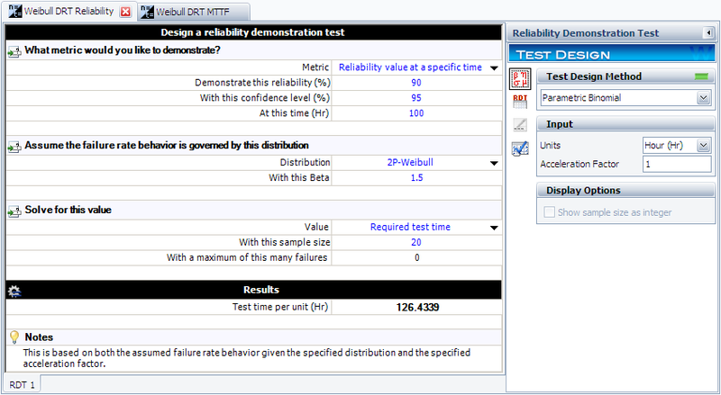
In this case, we will assume that we have 20 units to test, [math]\displaystyle{ n=20\,\! }[/math], and must determine the test time, [math]\displaystyle{ {{t}_{TEST}}\,\! }[/math]. We have already determined the value of the scale parameter, [math]\displaystyle{ \eta \,\! }[/math], in the previous example. Since we know the values of [math]\displaystyle{ n\,\! }[/math], [math]\displaystyle{ CL\,\! }[/math], [math]\displaystyle{ f\,\! }[/math], [math]\displaystyle{ \eta \,\! }[/math] and [math]\displaystyle{ \beta \,\! }[/math], it remains to solve the binomial equation with the Weibull distribution for [math]\displaystyle{ {{t}_{TEST}}\,\! }[/math]. This value is [math]\displaystyle{ {{t}_{TEST}}=126.4339\,\! }[/math] hours. This example solved in Weibull++ is shown next.


