The Gumbel/SEV Distribution: Difference between revisions
| (21 intermediate revisions by 4 users not shown) | |||
| Line 1: | Line 1: | ||
{{template:LDABOOK|16|The Gumbel/SEV Distribution}} | {{template:LDABOOK|16|The Gumbel/SEV Distribution}} | ||
The Gumbel distribution is also referred to as the Smallest Extreme Value (SEV) distribution or the Smallest Extreme Value (Type I) distribution. The Gumbel distribution's ''pdf'' is skewed to the left, unlike the Weibull distribution's ''pdf'', which is skewed to the right. The Gumbel distribution is appropriate for modeling strength, which is sometimes skewed to the left (few weak units in the lower tail, most units in the upper tail of the strength population). The Gumbel distribution could also be appropriate for modeling the life of products that experience very quick wear-out after reaching a certain age. The distribution of logarithms of times can often be modeled with the Gumbel distribution (in addition to the more common lognormal distribution), as discussed in Meeker and Escobar [[Appendix:_Life_Data_Analysis_References|[27]]]. | |||
The Gumbel distribution is also referred to as the Smallest Extreme Value (SEV) distribution or the Smallest Extreme Value (Type I) distribution. The Gumbel distribution's | |||
===Gumbel Probability Density Function=== | ===Gumbel Probability Density Function=== | ||
The | The ''pdf'' of the Gumbel distribution is given by: | ||
::<math>f(t)=\frac{1}{\sigma }{{e}^{z-{{e}^{z}}}}</math> | ::<math>f(t)=\frac{1}{\sigma }{{e}^{z-{{e}^{z}}}}\,\!</math> | ||
::<math>f(t)\ge 0,\sigma >0</math> | ::<math>f(t)\ge 0,\sigma >0\,\!</math> | ||
where: | where: | ||
::<math>z=\frac{t-\mu }{\sigma }</math> | ::<math>z=\frac{t-\mu }{\sigma }\,\!</math> | ||
and: | and: | ||
| Line 19: | Line 18: | ||
& \mu = \text{location parameter} \\ | & \mu = \text{location parameter} \\ | ||
& \sigma = \text{scale parameter} | & \sigma = \text{scale parameter} | ||
\end{align}</math> | \end{align}\,\!</math> | ||
=== | ===Gumbel Mean, Median and Mode=== | ||
The Gumbel mean or MTTF is: | The Gumbel mean or MTTF is: | ||
::<math>\overline{T}=\mu -\sigma \gamma </math> | ::<math>\overline{T}=\mu -\sigma \gamma \,\!</math> | ||
where | where <math>\gamma \approx 0.5772\,\!</math> (Euler's constant). | ||
The mode of the Gumbel distribution is: | The mode of the Gumbel distribution is: | ||
::<math>\tilde{T}=\mu </math> | ::<math>\tilde{T}=\mu \,\!</math> | ||
The median of the Gumbel distribution is: | The median of the Gumbel distribution is: | ||
::<math>\widehat{T}=\mu +\sigma \ln (\ln (2))</math> | ::<math>\widehat{T}=\mu +\sigma \ln (\ln (2))\,\!</math> | ||
=== | ===Gumbel Standard Deviation=== | ||
The standard deviation for the Gumbel distribution is given by: | The standard deviation for the Gumbel distribution is given by: | ||
::<math>{{\sigma }_{T}}=\sigma \pi \frac{\sqrt{6}}{6}</math> | ::<math>{{\sigma }_{T}}=\sigma \pi \frac{\sqrt{6}}{6}\,\!</math> | ||
=== | ===Gumbel Reliability Function=== | ||
The reliability for a mission of time | The reliability for a mission of time <math>t\,\!</math> for the Gumbel distribution is given by: | ||
::<math>R(t)={{e}^{-{{e}^{z}}}}</math> | ::<math>R(t)={{e}^{-{{e}^{z}}}}\,\!</math> | ||
The unreliability function is given by: | The unreliability function is given by: | ||
::<math>F(t)=1-{{e}^{-{{e}^{z}}}}</math> | ::<math>F(t)=1-{{e}^{-{{e}^{z}}}}\,\!</math> | ||
=== | ===Gumbel Reliable Life=== | ||
The Gumbel reliable life is given by: | The Gumbel reliable life is given by: | ||
::<math>{{t}_{R}}=\mu +\sigma [\ln (-\ln (R))]</math> | ::<math>\begin{align} | ||
{{t}_{R}}=\mu +\sigma [\ln (-\ln (R))] | |||
\end{align}\,\!</math> | |||
=== | ===Gumbel Failure Rate Function=== | ||
The instantaneous Gumbel failure rate is given by: | The instantaneous Gumbel failure rate is given by: | ||
::<math>\lambda =\frac{{{e}^{z}}}{\sigma }</math> | ::<math>\lambda =\frac{{{e}^{z}}}{\sigma }\,\!</math> | ||
==Characteristics of the Gumbel Distribution== | ==Characteristics of the Gumbel Distribution== | ||
Some of the specific characteristics of the Gumbel distribution are the following: | Some of the specific characteristics of the Gumbel distribution are the following: | ||
:* The shape of the Gumbel distribution is skewed to the left. The Gumbel | :* The shape of the Gumbel distribution is skewed to the left. The Gumbel ''pdf'' has no shape parameter. This means that the Gumbel ''pdf'' has only one shape, which does not change. | ||
:* The Gumbel | :* The Gumbel ''pdf'' has location parameter <math>\mu ,\,\!</math> which is equal to the mode <math>\tilde{T},\,\!</math> but it differs from median and mean. This is because the Gumbel distribution is not symmetrical about its <math>\mu \,\!</math>. | ||
:* As | :* As <math>\mu \,\!</math> decreases, the ''pdf'' is shifted to the left. | ||
:* As | :* As <math>\mu \,\!</math> increases, the ''pdf'' is shifted to the right. | ||
[[Image:WB.16 gumbel pdf.png|center| | [[Image:WB.16 gumbel pdf.png|center|350px| ]] | ||
:* As | :* As <math>\sigma \,\!</math> increases, the ''pdf'' spreads out and becomes shallower. | ||
:* As | :* As <math>\sigma \,\!</math> decreases, the ''pdf'' becomes taller and narrower. | ||
:* For | :* For <math>T=\pm \infty ,\,\!</math> ''pdf''=0. For <math>T=\mu \,\!</math>, the ''pdf'' reaches its maximum point <math>\frac{1}{\sigma e}\,\!</math> | ||
[[Image:WB.16 effect of sigma.png|center| | [[Image:WB.16 effect of sigma.png|center|350px| ]] | ||
:* The points of inflection of the | :* The points of inflection of the ''pdf'' graph are <math>T=\mu \pm \sigma \ln (\tfrac{3\pm \sqrt{5}}{2})\,\!</math> or <math>T\approx \mu \pm \sigma 0.96242\,\!</math>. | ||
:* If times follow the Weibull distribution, then the logarithm of times follow a Gumbel distribution. If | :* If times follow the Weibull distribution, then the logarithm of times follow a Gumbel distribution. If <math>{{t}_{i}}\,\!</math> follows a Weibull distribution with <math>\beta \,\!</math> and <math>\eta \,\!</math>, then the <math>Ln({{t}_{i}})\,\!</math> follows a Gumbel distribution with <math>\mu =\ln (\eta )\,\!</math> and <math>\sigma =\tfrac{1}{\beta }\,\!</math>, as discussed in [[Appendix:_Life_Data_Analysis_References|[32]]]. | ||
==Probability Paper== | ==Probability Paper== | ||
The form of the Gumbel probability paper is based on a linearization of the | The form of the Gumbel probability paper is based on a linearization of the ''cdf''. From the unreliabililty equation, we know: | ||
::<math>z=\ln (-\ln (1-F))</math> | ::<math>\begin{align} | ||
z=\ln (-\ln (1-F)) | |||
\end{align}\,\!</math> | |||
using the equation for ''z'', we get: | using the equation for ''z'', we get: | ||
::<math>\frac{t-\mu }{\sigma }=\ln (-\ln (1-F))</math> | ::<math>\frac{t-\mu }{\sigma }=\ln (-\ln (1-F))\,\!</math> | ||
Then: | Then: | ||
::<math>\ln (-\ln (1-F))=-\frac{\mu }{\sigma }+\frac{1}{\sigma }t</math> | ::<math>\ln (-\ln (1-F))=-\frac{\mu }{\sigma }+\frac{1}{\sigma }t\,\!</math> | ||
Now let: | Now let: | ||
::<math>y=\ln (-\ln (1-F))</math> | ::<math>\begin{align} | ||
y=\ln (-\ln (1-F)) | |||
\end{align}\,\!</math> | |||
::<math>x=t</math> | ::<math>\begin{align} | ||
x=t | |||
\end{align}\,\!</math> | |||
and: | and: | ||
| Line 103: | Line 110: | ||
& a= & -\frac{\mu }{\sigma } \\ | & a= & -\frac{\mu }{\sigma } \\ | ||
& b= & \frac{1}{\sigma } | & b= & \frac{1}{\sigma } | ||
\end{align}</math> | \end{align}\,\!</math> | ||
which results in the linear equation of: | which results in the linear equation of: | ||
::<math>y=a+bx</math> | ::<math>\begin{align} | ||
y=a+bx | |||
\end{align}\,\!</math> | |||
The Gumbel probability paper resulting from this linearized | The Gumbel probability paper resulting from this linearized ''cdf'' function is shown next. | ||
[[Image:WB.16 probability gumbel.png|center| | [[Image:WB.16 probability gumbel.png|center|400px| ]] | ||
For <math>z=0\,\!</math>, <math>t=\mu \,\!</math> and <math>R(t)={{e}^{-{{e}^{0}}}}\approx 0.3678\,\!</math> (63.21% unreliability). For <math>z=1\,\!</math>, <math>\sigma =T-\mu \,\!</math> and <math>R(t)={{e}^{-{{e}^{1}}}}\approx 0.0659.\,\!</math> To read <math>\mu \,\!</math> from the plot, find the time value that corresponds to the intersection of the probability plot with the 63.21% unreliability line. To read <math>\sigma \,\!</math> from the plot, find the time value that corresponds to the intersection of the probability plot with the 93.40% unreliability line, then take the difference between this time value and the <math>\mu \,\!</math> value. | |||
==Confidence Bounds== | ==Confidence Bounds== | ||
This section presents the method used by the application to estimate the different types of confidence bounds for data that follow the Gumbel distribution. The complete derivations were presented in detail (for a general function) in [[Confidence Bounds]]. Only Fisher Matrix confidence bounds are available for the Gumbel distribution. | This section presents the method used by the application to estimate the different types of confidence bounds for data that follow the Gumbel distribution. The complete derivations were presented in detail (for a general function) in [[Confidence Bounds]]. Only Fisher Matrix confidence bounds are available for the Gumbel distribution. | ||
===Bounds on the Parameters=== | ===Bounds on the Parameters=== | ||
The lower and upper bounds on the mean, | The lower and upper bounds on the mean, <math>\widehat{\mu }\,\!</math>, are estimated from: | ||
::<math>\begin{align} | ::<math>\begin{align} | ||
& {{\mu }_{U}}= & \widehat{\mu }+{{K}_{\alpha }}\sqrt{Var(\widehat{\mu })}\text{ (upper bound)} \\ | & {{\mu }_{U}}= & \widehat{\mu }+{{K}_{\alpha }}\sqrt{Var(\widehat{\mu })}\text{ (upper bound)} \\ | ||
& {{\mu }_{L}}= & \widehat{\mu }-{{K}_{\alpha }}\sqrt{Var(\widehat{\mu })}\text{ (lower bound)} | & {{\mu }_{L}}= & \widehat{\mu }-{{K}_{\alpha }}\sqrt{Var(\widehat{\mu })}\text{ (lower bound)} | ||
\end{align}</math> | \end{align}\,\!</math> | ||
Since the standard deviation, <math>\widehat{\sigma }\,\!</math>, must be positive, then <math>\ln (\widehat{\sigma })\,\!</math> is treated as normally distributed, and the bounds are estimated from: | |||
Since the standard deviation, | |||
::<math>\begin{align} | ::<math>\begin{align} | ||
& {{\sigma }_{U}}= & \widehat{\sigma }\cdot {{e}^{\tfrac{{{K}_{\alpha }}\sqrt{Var(\widehat{\sigma })}}{{{\widehat{\sigma }}_{T}}}}}\text{ (upper bound)} \\ | & {{\sigma }_{U}}= & \widehat{\sigma }\cdot {{e}^{\tfrac{{{K}_{\alpha }}\sqrt{Var(\widehat{\sigma })}}{{{\widehat{\sigma }}_{T}}}}}\text{ (upper bound)} \\ | ||
& {{\sigma }_{L}}= & \frac{\widehat{\sigma }}{{{e}^{\tfrac{{{K}_{\alpha }}\sqrt{Var(\widehat{\sigma })}}{\widehat{\sigma }}}}}\text{ (lower bound)} | & {{\sigma }_{L}}= & \frac{\widehat{\sigma }}{{{e}^{\tfrac{{{K}_{\alpha }}\sqrt{Var(\widehat{\sigma })}}{\widehat{\sigma }}}}}\text{ (lower bound)} | ||
\end{align}</math> | \end{align}\,\!</math> | ||
where | where <math>{{K}_{\alpha }}\,\!</math> is defined by: | ||
::<math>\alpha =\frac{1}{\sqrt{2\pi }}\int_{{{K}_{\alpha }}}^{\infty }{{e}^{-\tfrac{{{t}^{2}}}{2}}}dt=1-\Phi ({{K}_{\alpha }})</math> | ::<math>\alpha =\frac{1}{\sqrt{2\pi }}\int_{{{K}_{\alpha }}}^{\infty }{{e}^{-\tfrac{{{t}^{2}}}{2}}}dt=1-\Phi ({{K}_{\alpha }})\,\!</math> | ||
If <math>\delta \,\!</math> is the confidence level, then <math>\alpha =\tfrac{1-\delta }{2}\,\!</math> for the two-sided bounds, and <math>\alpha =1-\delta \,\!</math> for the one-sided bounds. | |||
The variances and covariances of <math>\widehat{\mu }\,\!</math> and <math>\widehat{\sigma }\,\!</math> are estimated from the Fisher matrix as follows: | |||
The variances and covariances of | |||
::<math>\left( \begin{matrix} | ::<math>\left( \begin{matrix} | ||
| Line 153: | Line 157: | ||
{} & {} \\ | {} & {} \\ | ||
-\tfrac{{{\partial }^{2}}\Lambda }{\partial \mu \partial \sigma } & -\tfrac{{{\partial }^{2}}\Lambda }{\partial {{\sigma }^{2}}} \\ | -\tfrac{{{\partial }^{2}}\Lambda }{\partial \mu \partial \sigma } & -\tfrac{{{\partial }^{2}}\Lambda }{\partial {{\sigma }^{2}}} \\ | ||
\end{matrix} \right)_{\mu =\widehat{\mu },\sigma =\widehat{\sigma }}^{-1}</math> | \end{matrix} \right)_{\mu =\widehat{\mu },\sigma =\widehat{\sigma }}^{-1}\,\!</math> | ||
<math>\Lambda \,\!</math> is the log-likelihood function of the Gumbel distribution, described in [[Parameter Estimation]] and [[Appendix:_Log-Likelihood_Equations|Appendix D]]. | |||
<math>\Lambda </math> | |||
===Bounds on Reliability=== | ===Bounds on Reliability=== | ||
The reliability of the Gumbel distribution is given by: | The reliability of the Gumbel distribution is given by: | ||
::<math>\widehat{R}(t;\hat{\mu },\hat{\sigma })={{e}^{-{{e}^{{\hat{z}}}}}}</math> | ::<math>\widehat{R}(t;\hat{\mu },\hat{\sigma })={{e}^{-{{e}^{{\hat{z}}}}}}\,\!</math> | ||
where: | where: | ||
::<math>\widehat{z}=\frac{t-\widehat{\mu }}{\widehat{\sigma }}</math> | ::<math>\widehat{z}=\frac{t-\widehat{\mu }}{\widehat{\sigma }}\,\!</math> | ||
The bounds on | The bounds on <math>z\,\!</math> are estimated from: | ||
::<math>\begin{align} | ::<math>\begin{align} | ||
& {{z}_{U}}= & \widehat{z}+{{K}_{\alpha }}\sqrt{Var(\widehat{z})} \\ | & {{z}_{U}}= & \widehat{z}+{{K}_{\alpha }}\sqrt{Var(\widehat{z})} \\ | ||
& {{z}_{L}}= & \widehat{z}-{{K}_{\alpha }}\sqrt{Var(\widehat{z})} | & {{z}_{L}}= & \widehat{z}-{{K}_{\alpha }}\sqrt{Var(\widehat{z})} | ||
\end{align}</math> | \end{align}\,\!</math> | ||
where: | where: | ||
::<math>Var(\widehat{z})={{\left( \frac{\partial z}{\partial \mu } \right)}^{2}}Var(\widehat{\mu })+{{\left( \frac{\partial z}{\partial \sigma } \right)}^{2}}Var(\widehat{\sigma })+2\left( \frac{\partial z}{\partial \mu } \right)\left( \frac{\partial z}{\partial \sigma } \right)Cov\left( \widehat{\mu },\widehat{\sigma } \right)</math> | ::<math>Var(\widehat{z})={{\left( \frac{\partial z}{\partial \mu } \right)}^{2}}Var(\widehat{\mu })+{{\left( \frac{\partial z}{\partial \sigma } \right)}^{2}}Var(\widehat{\sigma })+2\left( \frac{\partial z}{\partial \mu } \right)\left( \frac{\partial z}{\partial \sigma } \right)Cov\left( \widehat{\mu },\widehat{\sigma } \right)\,\!</math> | ||
or: | or: | ||
::<math>Var(\widehat{z})=\frac{1}{{{\widehat{\sigma }}^{2}}}\left[ Var(\widehat{\mu })+{{\widehat{z}}^{2}}Var(\widehat{\sigma })+2\cdot \widehat{z}\cdot Cov\left( \widehat{\mu },\widehat{\sigma } \right) \right]</math> | ::<math>Var(\widehat{z})=\frac{1}{{{\widehat{\sigma }}^{2}}}\left[ Var(\widehat{\mu })+{{\widehat{z}}^{2}}Var(\widehat{\sigma })+2\cdot \widehat{z}\cdot Cov\left( \widehat{\mu },\widehat{\sigma } \right) \right]\,\!</math> | ||
The upper and lower bounds on reliability are: | The upper and lower bounds on reliability are: | ||
| Line 188: | Line 190: | ||
& {{R}_{U}}= & {{e}^{-{{e}^{{{z}_{L}}}}}}\text{ (upper bound)} \\ | & {{R}_{U}}= & {{e}^{-{{e}^{{{z}_{L}}}}}}\text{ (upper bound)} \\ | ||
& {{R}_{L}}= & {{e}^{-{{e}^{{{z}_{U}}}}}}\text{ (lower bound)} | & {{R}_{L}}= & {{e}^{-{{e}^{{{z}_{U}}}}}}\text{ (lower bound)} | ||
\end{align}</math> | \end{align}\,\!</math> | ||
===Bounds on Time=== | ===Bounds on Time=== | ||
The bounds around time for a given Gumbel percentile (unreliability) are estimated by first solving the reliability equation with respect to time, as follows: | The bounds around time for a given Gumbel percentile (unreliability) are estimated by first solving the reliability equation with respect to time, as follows: | ||
::<math>\widehat{T}(\widehat{\mu },\widehat{\sigma })=\widehat{\mu }+\widehat{\sigma }z</math> | ::<math>\widehat{T}(\widehat{\mu },\widehat{\sigma })=\widehat{\mu }+\widehat{\sigma }z\,\!</math> | ||
where: | where: | ||
::<math>z=\ln (-\ln (R))</math> | ::<math>\begin{align} | ||
z=\ln (-\ln (R)) | |||
\end{align}\,\!</math> | |||
::<math>Var(\widehat{T})={{(\frac{\partial T}{\partial \mu })}^{2}}Var(\widehat{\mu })+2(\frac{\partial T}{\partial \mu })(\frac{\partial T}{\partial \sigma })Cov(\widehat{\mu },\widehat{\sigma })+{{(\frac{\partial T}{\partial \sigma })}^{2}}Var(\widehat{\sigma })</math> | ::<math>Var(\widehat{T})={{(\frac{\partial T}{\partial \mu })}^{2}}Var(\widehat{\mu })+2(\frac{\partial T}{\partial \mu })(\frac{\partial T}{\partial \sigma })Cov(\widehat{\mu },\widehat{\sigma })+{{(\frac{\partial T}{\partial \sigma })}^{2}}Var(\widehat{\sigma })\,\!</math> | ||
or: | or: | ||
::<math>Var(\widehat{T})=Var(\widehat{\mu })+2\widehat{z}Cov(\widehat{\mu },\widehat{\sigma })+{{\widehat{z}}^{2}}Var(\widehat{\sigma })</math> | ::<math>Var(\widehat{T})=Var(\widehat{\mu })+2\widehat{z}Cov(\widehat{\mu },\widehat{\sigma })+{{\widehat{z}}^{2}}Var(\widehat{\sigma })\,\!</math> | ||
The upper and lower bounds are then found by: | The upper and lower bounds are then found by: | ||
| Line 212: | Line 214: | ||
& {{T}_{U}}= & \hat{T}+{{K}_{\alpha }}\sqrt{Var(\hat{T})}\text{ (Upper bound)} \\ | & {{T}_{U}}= & \hat{T}+{{K}_{\alpha }}\sqrt{Var(\hat{T})}\text{ (Upper bound)} \\ | ||
& {{T}_{L}}= & \hat{T}-{{K}_{\alpha }}\sqrt{Var(\hat{T})}\text{ (Lower bound)} | & {{T}_{L}}= & \hat{T}-{{K}_{\alpha }}\sqrt{Var(\hat{T})}\text{ (Lower bound)} | ||
\end{align}</math> | \end{align}\,\!</math> | ||
==Example== | |||
{{:Gumbel_Distribution_Example}} | |||
Latest revision as of 17:12, 23 December 2015
The Gumbel distribution is also referred to as the Smallest Extreme Value (SEV) distribution or the Smallest Extreme Value (Type I) distribution. The Gumbel distribution's pdf is skewed to the left, unlike the Weibull distribution's pdf, which is skewed to the right. The Gumbel distribution is appropriate for modeling strength, which is sometimes skewed to the left (few weak units in the lower tail, most units in the upper tail of the strength population). The Gumbel distribution could also be appropriate for modeling the life of products that experience very quick wear-out after reaching a certain age. The distribution of logarithms of times can often be modeled with the Gumbel distribution (in addition to the more common lognormal distribution), as discussed in Meeker and Escobar [27].
Gumbel Probability Density Function
The pdf of the Gumbel distribution is given by:
- [math]\displaystyle{ f(t)=\frac{1}{\sigma }{{e}^{z-{{e}^{z}}}}\,\! }[/math]
- [math]\displaystyle{ f(t)\ge 0,\sigma \gt 0\,\! }[/math]
where:
- [math]\displaystyle{ z=\frac{t-\mu }{\sigma }\,\! }[/math]
and:
- [math]\displaystyle{ \begin{align} & \mu = \text{location parameter} \\ & \sigma = \text{scale parameter} \end{align}\,\! }[/math]
Gumbel Mean, Median and Mode
The Gumbel mean or MTTF is:
- [math]\displaystyle{ \overline{T}=\mu -\sigma \gamma \,\! }[/math]
where [math]\displaystyle{ \gamma \approx 0.5772\,\! }[/math] (Euler's constant).
The mode of the Gumbel distribution is:
- [math]\displaystyle{ \tilde{T}=\mu \,\! }[/math]
The median of the Gumbel distribution is:
- [math]\displaystyle{ \widehat{T}=\mu +\sigma \ln (\ln (2))\,\! }[/math]
Gumbel Standard Deviation
The standard deviation for the Gumbel distribution is given by:
- [math]\displaystyle{ {{\sigma }_{T}}=\sigma \pi \frac{\sqrt{6}}{6}\,\! }[/math]
Gumbel Reliability Function
The reliability for a mission of time [math]\displaystyle{ t\,\! }[/math] for the Gumbel distribution is given by:
- [math]\displaystyle{ R(t)={{e}^{-{{e}^{z}}}}\,\! }[/math]
The unreliability function is given by:
- [math]\displaystyle{ F(t)=1-{{e}^{-{{e}^{z}}}}\,\! }[/math]
Gumbel Reliable Life
The Gumbel reliable life is given by:
- [math]\displaystyle{ \begin{align} {{t}_{R}}=\mu +\sigma [\ln (-\ln (R))] \end{align}\,\! }[/math]
Gumbel Failure Rate Function
The instantaneous Gumbel failure rate is given by:
- [math]\displaystyle{ \lambda =\frac{{{e}^{z}}}{\sigma }\,\! }[/math]
Characteristics of the Gumbel Distribution
Some of the specific characteristics of the Gumbel distribution are the following:
- The shape of the Gumbel distribution is skewed to the left. The Gumbel pdf has no shape parameter. This means that the Gumbel pdf has only one shape, which does not change.
- The Gumbel pdf has location parameter [math]\displaystyle{ \mu ,\,\! }[/math] which is equal to the mode [math]\displaystyle{ \tilde{T},\,\! }[/math] but it differs from median and mean. This is because the Gumbel distribution is not symmetrical about its [math]\displaystyle{ \mu \,\! }[/math].
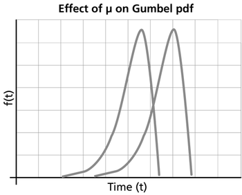
- As [math]\displaystyle{ \mu \,\! }[/math] decreases, the pdf is shifted to the left.
- As [math]\displaystyle{ \mu \,\! }[/math] increases, the pdf is shifted to the right.
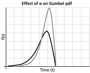
- As [math]\displaystyle{ \sigma \,\! }[/math] increases, the pdf spreads out and becomes shallower.
- As [math]\displaystyle{ \sigma \,\! }[/math] decreases, the pdf becomes taller and narrower.
- For [math]\displaystyle{ T=\pm \infty ,\,\! }[/math] pdf=0. For [math]\displaystyle{ T=\mu \,\! }[/math], the pdf reaches its maximum point [math]\displaystyle{ \frac{1}{\sigma e}\,\! }[/math]
- The points of inflection of the pdf graph are [math]\displaystyle{ T=\mu \pm \sigma \ln (\tfrac{3\pm \sqrt{5}}{2})\,\! }[/math] or [math]\displaystyle{ T\approx \mu \pm \sigma 0.96242\,\! }[/math].
- If times follow the Weibull distribution, then the logarithm of times follow a Gumbel distribution. If [math]\displaystyle{ {{t}_{i}}\,\! }[/math] follows a Weibull distribution with [math]\displaystyle{ \beta \,\! }[/math] and [math]\displaystyle{ \eta \,\! }[/math], then the [math]\displaystyle{ Ln({{t}_{i}})\,\! }[/math] follows a Gumbel distribution with [math]\displaystyle{ \mu =\ln (\eta )\,\! }[/math] and [math]\displaystyle{ \sigma =\tfrac{1}{\beta }\,\! }[/math], as discussed in [32].
Probability Paper
The form of the Gumbel probability paper is based on a linearization of the cdf. From the unreliabililty equation, we know:
- [math]\displaystyle{ \begin{align} z=\ln (-\ln (1-F)) \end{align}\,\! }[/math]
using the equation for z, we get:
- [math]\displaystyle{ \frac{t-\mu }{\sigma }=\ln (-\ln (1-F))\,\! }[/math]
Then:
- [math]\displaystyle{ \ln (-\ln (1-F))=-\frac{\mu }{\sigma }+\frac{1}{\sigma }t\,\! }[/math]
Now let:
- [math]\displaystyle{ \begin{align} y=\ln (-\ln (1-F)) \end{align}\,\! }[/math]
- [math]\displaystyle{ \begin{align} x=t \end{align}\,\! }[/math]
and:
- [math]\displaystyle{ \begin{align} & a= & -\frac{\mu }{\sigma } \\ & b= & \frac{1}{\sigma } \end{align}\,\! }[/math]
which results in the linear equation of:
- [math]\displaystyle{ \begin{align} y=a+bx \end{align}\,\! }[/math]
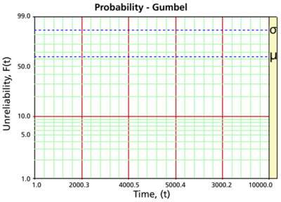
The Gumbel probability paper resulting from this linearized cdf function is shown next.
For [math]\displaystyle{ z=0\,\! }[/math], [math]\displaystyle{ t=\mu \,\! }[/math] and [math]\displaystyle{ R(t)={{e}^{-{{e}^{0}}}}\approx 0.3678\,\! }[/math] (63.21% unreliability). For [math]\displaystyle{ z=1\,\! }[/math], [math]\displaystyle{ \sigma =T-\mu \,\! }[/math] and [math]\displaystyle{ R(t)={{e}^{-{{e}^{1}}}}\approx 0.0659.\,\! }[/math] To read [math]\displaystyle{ \mu \,\! }[/math] from the plot, find the time value that corresponds to the intersection of the probability plot with the 63.21% unreliability line. To read [math]\displaystyle{ \sigma \,\! }[/math] from the plot, find the time value that corresponds to the intersection of the probability plot with the 93.40% unreliability line, then take the difference between this time value and the [math]\displaystyle{ \mu \,\! }[/math] value.
Confidence Bounds
This section presents the method used by the application to estimate the different types of confidence bounds for data that follow the Gumbel distribution. The complete derivations were presented in detail (for a general function) in Confidence Bounds. Only Fisher Matrix confidence bounds are available for the Gumbel distribution.
Bounds on the Parameters
The lower and upper bounds on the mean, [math]\displaystyle{ \widehat{\mu }\,\! }[/math], are estimated from:
- [math]\displaystyle{ \begin{align} & {{\mu }_{U}}= & \widehat{\mu }+{{K}_{\alpha }}\sqrt{Var(\widehat{\mu })}\text{ (upper bound)} \\ & {{\mu }_{L}}= & \widehat{\mu }-{{K}_{\alpha }}\sqrt{Var(\widehat{\mu })}\text{ (lower bound)} \end{align}\,\! }[/math]
Since the standard deviation, [math]\displaystyle{ \widehat{\sigma }\,\! }[/math], must be positive, then [math]\displaystyle{ \ln (\widehat{\sigma })\,\! }[/math] is treated as normally distributed, and the bounds are estimated from:
- [math]\displaystyle{ \begin{align} & {{\sigma }_{U}}= & \widehat{\sigma }\cdot {{e}^{\tfrac{{{K}_{\alpha }}\sqrt{Var(\widehat{\sigma })}}{{{\widehat{\sigma }}_{T}}}}}\text{ (upper bound)} \\ & {{\sigma }_{L}}= & \frac{\widehat{\sigma }}{{{e}^{\tfrac{{{K}_{\alpha }}\sqrt{Var(\widehat{\sigma })}}{\widehat{\sigma }}}}}\text{ (lower bound)} \end{align}\,\! }[/math]
where [math]\displaystyle{ {{K}_{\alpha }}\,\! }[/math] is defined by:
- [math]\displaystyle{ \alpha =\frac{1}{\sqrt{2\pi }}\int_{{{K}_{\alpha }}}^{\infty }{{e}^{-\tfrac{{{t}^{2}}}{2}}}dt=1-\Phi ({{K}_{\alpha }})\,\! }[/math]
If [math]\displaystyle{ \delta \,\! }[/math] is the confidence level, then [math]\displaystyle{ \alpha =\tfrac{1-\delta }{2}\,\! }[/math] for the two-sided bounds, and [math]\displaystyle{ \alpha =1-\delta \,\! }[/math] for the one-sided bounds.
The variances and covariances of [math]\displaystyle{ \widehat{\mu }\,\! }[/math] and [math]\displaystyle{ \widehat{\sigma }\,\! }[/math] are estimated from the Fisher matrix as follows:
- [math]\displaystyle{ \left( \begin{matrix} \widehat{Var}\left( \widehat{\mu } \right) & \widehat{Cov}\left( \widehat{\mu },\widehat{\sigma } \right) \\ \widehat{Cov}\left( \widehat{\mu },\widehat{\sigma } \right) & \widehat{Var}\left( \widehat{\sigma } \right) \\ \end{matrix} \right)=\left( \begin{matrix} -\tfrac{{{\partial }^{2}}\Lambda }{\partial {{\mu }^{2}}} & -\tfrac{{{\partial }^{2}}\Lambda }{\partial \mu \partial \sigma } \\ {} & {} \\ -\tfrac{{{\partial }^{2}}\Lambda }{\partial \mu \partial \sigma } & -\tfrac{{{\partial }^{2}}\Lambda }{\partial {{\sigma }^{2}}} \\ \end{matrix} \right)_{\mu =\widehat{\mu },\sigma =\widehat{\sigma }}^{-1}\,\! }[/math]
[math]\displaystyle{ \Lambda \,\! }[/math] is the log-likelihood function of the Gumbel distribution, described in Parameter Estimation and Appendix D.
Bounds on Reliability
The reliability of the Gumbel distribution is given by:
- [math]\displaystyle{ \widehat{R}(t;\hat{\mu },\hat{\sigma })={{e}^{-{{e}^{{\hat{z}}}}}}\,\! }[/math]
where:
- [math]\displaystyle{ \widehat{z}=\frac{t-\widehat{\mu }}{\widehat{\sigma }}\,\! }[/math]
The bounds on [math]\displaystyle{ z\,\! }[/math] are estimated from:
- [math]\displaystyle{ \begin{align} & {{z}_{U}}= & \widehat{z}+{{K}_{\alpha }}\sqrt{Var(\widehat{z})} \\ & {{z}_{L}}= & \widehat{z}-{{K}_{\alpha }}\sqrt{Var(\widehat{z})} \end{align}\,\! }[/math]
where:
- [math]\displaystyle{ Var(\widehat{z})={{\left( \frac{\partial z}{\partial \mu } \right)}^{2}}Var(\widehat{\mu })+{{\left( \frac{\partial z}{\partial \sigma } \right)}^{2}}Var(\widehat{\sigma })+2\left( \frac{\partial z}{\partial \mu } \right)\left( \frac{\partial z}{\partial \sigma } \right)Cov\left( \widehat{\mu },\widehat{\sigma } \right)\,\! }[/math]
or:
- [math]\displaystyle{ Var(\widehat{z})=\frac{1}{{{\widehat{\sigma }}^{2}}}\left[ Var(\widehat{\mu })+{{\widehat{z}}^{2}}Var(\widehat{\sigma })+2\cdot \widehat{z}\cdot Cov\left( \widehat{\mu },\widehat{\sigma } \right) \right]\,\! }[/math]
The upper and lower bounds on reliability are:
- [math]\displaystyle{ \begin{align} & {{R}_{U}}= & {{e}^{-{{e}^{{{z}_{L}}}}}}\text{ (upper bound)} \\ & {{R}_{L}}= & {{e}^{-{{e}^{{{z}_{U}}}}}}\text{ (lower bound)} \end{align}\,\! }[/math]
Bounds on Time
The bounds around time for a given Gumbel percentile (unreliability) are estimated by first solving the reliability equation with respect to time, as follows:
- [math]\displaystyle{ \widehat{T}(\widehat{\mu },\widehat{\sigma })=\widehat{\mu }+\widehat{\sigma }z\,\! }[/math]
where:
- [math]\displaystyle{ \begin{align} z=\ln (-\ln (R)) \end{align}\,\! }[/math]
- [math]\displaystyle{ Var(\widehat{T})={{(\frac{\partial T}{\partial \mu })}^{2}}Var(\widehat{\mu })+2(\frac{\partial T}{\partial \mu })(\frac{\partial T}{\partial \sigma })Cov(\widehat{\mu },\widehat{\sigma })+{{(\frac{\partial T}{\partial \sigma })}^{2}}Var(\widehat{\sigma })\,\! }[/math]
or:
- [math]\displaystyle{ Var(\widehat{T})=Var(\widehat{\mu })+2\widehat{z}Cov(\widehat{\mu },\widehat{\sigma })+{{\widehat{z}}^{2}}Var(\widehat{\sigma })\,\! }[/math]
The upper and lower bounds are then found by:
- [math]\displaystyle{ \begin{align} & {{T}_{U}}= & \hat{T}+{{K}_{\alpha }}\sqrt{Var(\hat{T})}\text{ (Upper bound)} \\ & {{T}_{L}}= & \hat{T}-{{K}_{\alpha }}\sqrt{Var(\hat{T})}\text{ (Lower bound)} \end{align}\,\! }[/math]
Example
Verify using Monte Carlo simulation that if [math]\displaystyle{ {{t}_{i}}\,\! }[/math] follows a Weibull distribution with [math]\displaystyle{ \beta \,\! }[/math] and [math]\displaystyle{ \eta \,\! }[/math], then the [math]\displaystyle{ Ln({{t}_{i}})\,\! }[/math] follows a Gumbel distribution with [math]\displaystyle{ \mu =\ln (\eta )\,\! }[/math] and [math]\displaystyle{ \sigma =1/\beta )\,\! }[/math].
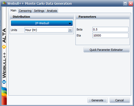
Let us assume that [math]\displaystyle{ {{t}_{i}}\,\! }[/math] follows a Weibull distribution with [math]\displaystyle{ \beta =0.5\,\! }[/math] and [math]\displaystyle{ \eta =10000\,\! }[/math]. The Monte Carlo simulation tool in Weibull++ can be used to generate a set of random numbers that follow a Weibull distribution with the specified parameters. The following picture shows the Main tab of the Monte Carlo Data Generation utility.
On the Settings tab, set the number of points to 100 and click Generate. This creates a new data sheet in the folio that contains random time values [math]\displaystyle{ {{t}_{i}}\,\! }[/math].
Insert a new data sheet in the folio and enter the corresponding [math]\displaystyle{ Ln({{t}_{i}})\,\! }[/math] values of the time values generated by the Monte Carlo simulation. Delete any negative values, if there are any, because Weibull++ expects the time values to be positive. After obtaining the [math]\displaystyle{ Ln({{t}_{i}})\,\! }[/math] values, analyze the data sheet using the Gumbel distribution and the MLE parameter estimation method. The estimated parameters are (your results may vary due to the random numbers generated by simulation):
- [math]\displaystyle{ \begin{align} & \hat{\mu }= & 9.3816 \\ & \hat{\sigma }= & 1.9717 \end{align}\,\! }[/math]
Because [math]\displaystyle{ \ln (\eta )= 9.2103\,\! }[/math] ( [math]\displaystyle{ \simeq 9.3816\,\! }[/math] ) and [math]\displaystyle{ 1/\beta =2\,\! }[/math] [math]\displaystyle{ (\simeq 1.9717)\,\! }[/math], then this simulation verifies that [math]\displaystyle{ Ln({{t}_{i}})\,\! }[/math] follows a Gumbel distribution with [math]\displaystyle{ \mu =\ln (\eta )\,\! }[/math] and [math]\displaystyle{ \delta =1/\beta \,\! }[/math].
Note: This example illustrates a property of the Gumbel distribution; it is not meant to be a formal proof.


