Example: Lognormal Distribution Probability Plot: Difference between revisions
Kate Racaza (talk | contribs) (proofread) |
Lisa Hacker (talk | contribs) No edit summary |
||
| (4 intermediate revisions by 2 users not shown) | |||
| Line 1: | Line 1: | ||
<noinclude>{{Banner Weibull Examples}} | <noinclude>{{Banner Weibull Examples}} | ||
''This example appears in the [ | ''This example appears in the [https://help.reliasoft.com/reference/life_data_analysis Life data analysis reference]''. | ||
</noinclude> | </noinclude> | ||
8 units are put on a life test and tested to failure. The failures occurred at 45, 140, 260, 500, 850, 1400, 3000, and 9000 hours. Estimate the parameters for the lognormal distribution using probability plotting. | |||
'''Solution''' | '''Solution''' | ||
| Line 21: | Line 20: | ||
\text{3000} & \text{79}\text{.89 }\!\!%\!\!\text{ } \\ | \text{3000} & \text{79}\text{.89 }\!\!%\!\!\text{ } \\ | ||
\text{9000} & \text{91}\text{.70 }\!\!%\!\!\text{ } \\ | \text{9000} & \text{91}\text{.70 }\!\!%\!\!\text{ } \\ | ||
\end{matrix}</math></center> | \end{matrix}\,\!</math></center> | ||
| Line 32: | Line 31: | ||
[[Image:WB.10 lpp3.png|center|420px| ]] | [[Image:WB.10 lpp3.png|center|420px| ]] | ||
The natural logarithm of the time where the fitted line intersects is equivalent to | The natural logarithm of the time where the fitted line intersects is equivalent to <math>{\mu }'\,\!</math>. In this case, <math>{\mu }'=6.45\,\!</math>. The value for <math>{{\sigma }_{{{T}'}}}\,\!</math> is equal to the difference between the natural logarithms of the times where the fitted line crosses <math>Q(t)=50%\,\!</math> and <math>Q(t)=15.85%.\,\!</math> At <math>Q(t)=15.85%\,\!</math>, ln <math>(t)=4.55\,\!</math>. Therefore, <math>{\sigma'}=6.45-4.55=1.9\,\!</math>. | ||
Latest revision as of 21:45, 18 September 2023
New format available! This reference is now available in a new format that offers faster page load, improved display for calculations and images and more targeted search.
As of January 2024, this Reliawiki page will not continue to be updated. Please update all links and bookmarks to the latest references at Weibull examples and Weibull reference examples.
This example appears in the Life data analysis reference.
8 units are put on a life test and tested to failure. The failures occurred at 45, 140, 260, 500, 850, 1400, 3000, and 9000 hours. Estimate the parameters for the lognormal distribution using probability plotting.
Solution
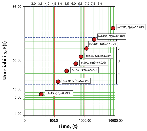
In order to plot the points for the probability plot, the appropriate unreliability estimate values must be obtained. These will be estimated through the use of median ranks, which can be obtained from statistical tables or the Quick Statistical Reference in Weibull++. The following table shows the times-to-failure and the appropriate median rank values for this example:
These points may now be plotted on normal probability plotting paper as shown in the next figure.
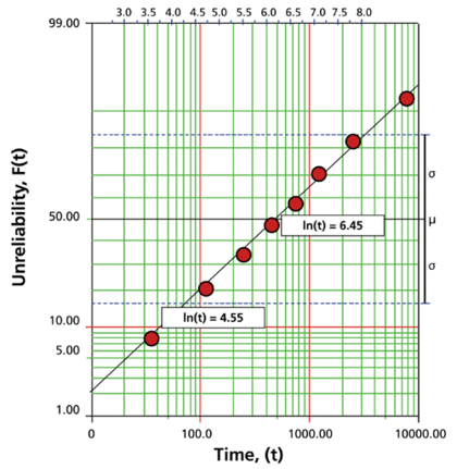
Draw the best possible line through the plot points. The time values where this line intersects the 15.85% and 50% unreliability values should be projected up to the logarithmic scale, as shown in the following plot.
The natural logarithm of the time where the fitted line intersects is equivalent to [math]\displaystyle{ {\mu }'\,\! }[/math]. In this case, [math]\displaystyle{ {\mu }'=6.45\,\! }[/math]. The value for [math]\displaystyle{ {{\sigma }_{{{T}'}}}\,\! }[/math] is equal to the difference between the natural logarithms of the times where the fitted line crosses [math]\displaystyle{ Q(t)=50%\,\! }[/math] and [math]\displaystyle{ Q(t)=15.85%.\,\! }[/math] At [math]\displaystyle{ Q(t)=15.85%\,\! }[/math], ln [math]\displaystyle{ (t)=4.55\,\! }[/math]. Therefore, [math]\displaystyle{ {\sigma'}=6.45-4.55=1.9\,\! }[/math].


