Template:Example: Likelihood Ratio Bounds on Parameters: Difference between revisions
No edit summary |
No edit summary |
||
| (8 intermediate revisions by 4 users not shown) | |||
| Line 1: | Line 1: | ||
'''Likelihood Ratio Bounds on Parameters''' | '''Likelihood Ratio Bounds on Parameters''' | ||
Five units were put on a reliability test and experienced failures at 10, 20, 30, 40 and 50 hours. Assuming a Weibull distribution, the MLE parameter estimates are calculated to be <math>\widehat{\beta }=2.2938</math> and <math>\widehat{\eta }=33.9428.</math> Calculate the 90% two-sided confidence bounds on these parameters using the likelihood ratio method. | Five units were put on a reliability test and experienced failures at 10, 20, 30, 40 and 50 hours. Assuming a Weibull distribution, the MLE parameter estimates are calculated to be <math>\widehat{\beta }=2.2938\,\!</math> and <math>\widehat{\eta }=33.9428.\,\!</math> Calculate the 90% two-sided confidence bounds on these parameters using the likelihood ratio method. | ||
'''Solution''' | |||
The first step is to calculate the likelihood function for the parameter estimates: | The first step is to calculate the likelihood function for the parameter estimates: | ||
| Line 13: | Line 13: | ||
\\ | \\ | ||
L(\widehat{\beta },\widehat{\eta })= & 1.714714\times {{10}^{-9}} | L(\widehat{\beta },\widehat{\eta })= & 1.714714\times {{10}^{-9}} | ||
\end{align}</math> | \end{align}\,\!</math> | ||
where <math>{{x}_{i}}\,\!</math> are the original time-to-failure data points. We can now rearrange the likelihood ratio equation to the form: | |||
< | ::<math>L(\beta ,\eta )-L(\widehat{\beta },\widehat{\eta })\cdot {{e}^{\tfrac{-\chi _{\alpha ;1}^{2}}{2}}}=0\,\!</math> | ||
Since our specified confidence level, <math>\delta\,\!</math>, is 90%, we can calculate the value of the chi-squared statistic, <math>\chi _{0.9;1}^{2}=2.705543.\,\!</math> We then substitute this information into the equation: | |||
::<math>\begin{align} | ::<math>\begin{align} | ||
L(\beta ,\eta )-L(\widehat{\beta },\widehat{\eta })\cdot {{e}^{\tfrac{-\chi _{\ | L(\beta ,\eta )-L(\widehat{\beta },\widehat{\eta })\cdot {{e}^{\tfrac{-\chi _{\alpha ;1}^{2}}{2}}}= & 0 \\ | ||
\\ | \\ | ||
L(\beta ,\eta )-1.714714\times {{10}^{-9}}\cdot {{e}^{\tfrac{-2.705543}{2}}}= & 0 \\ | L(\beta ,\eta )-1.714714\times {{10}^{-9}}\cdot {{e}^{\tfrac{-2.705543}{2}}}= & 0 \\ | ||
\\ | \\ | ||
L(\beta ,\eta )-4.432926\cdot {{10}^{-10}}= & 0 | L(\beta ,\eta )-4.432926\cdot {{10}^{-10}}= & 0 | ||
\end{align}</math> | \end{align}\,\!</math> | ||
The next step is to find the set of values of <math>\beta\,\!</math> and <math>\eta\,\!</math> that satisfy this equation, or find the values of <math>\beta\,\!</math> and <math>\eta\,\!</math> such that <math>L(\beta ,\eta )=4.432926\cdot {{10}^{-10}}.\,\!</math> | |||
The solution is an iterative process that requires setting the value of < | The solution is an iterative process that requires setting the value of <math>\beta\,\!</math> and finding the appropriate values of <math>\eta\,\!</math>, and vice versa. The following table gives values of <math>\beta\,\!</math> based on given values of <math>\eta\,\!</math>. | ||
[[Image:Confidencechart1.png|center|300px]] | |||
These data are represented graphically in the following contour plot: | |||
[[Image:weibull parameter contour plot.png|center|425px]] | |||
(Note that this plot is generated with degrees of freedom <math>k = 1\,\!</math>, as we are only determining bounds on one parameter. The contour plots generated in Weibull++ are done with degrees of freedom <math>k = 2\,\!</math>, for use in comparing both parameters simultaneously.) As can be determined from the table, the lowest calculated value for <math>\beta\,\!</math> is 1.142, while the highest is 3.950. These represent the two-sided 90% confidence limits on this parameter. Since solutions for the equation do not exist for values of <math>\eta\,\!</math> below 23 or above 50, these can be considered the 90% confidence limits for this parameter. In order to obtain more accurate values for the confidence limits on <math>\eta\,\!</math>, we can perform the same procedure as before, but finding the two values of <math>\eta\,\!</math> that correspond with a given value of <math>\beta\,\!</math> Using this method, we find that the 90% confidence limits on <math>\eta\,\!</math> are 22.474 and 49.967, which are close to the initial estimates of 23 and 50. | |||
Note that the points where <math>\beta\,\!</math> are maximized and minimized do not necessarily correspond with the points where <math>\eta\,\!</math> are maximized and minimized. This is due to the fact that the contour plot is not symmetrical, so that the parameters will have their extremes at different points. | |||
Latest revision as of 17:53, 21 December 2015
Likelihood Ratio Bounds on Parameters
Five units were put on a reliability test and experienced failures at 10, 20, 30, 40 and 50 hours. Assuming a Weibull distribution, the MLE parameter estimates are calculated to be [math]\displaystyle{ \widehat{\beta }=2.2938\,\! }[/math] and [math]\displaystyle{ \widehat{\eta }=33.9428.\,\! }[/math] Calculate the 90% two-sided confidence bounds on these parameters using the likelihood ratio method.
Solution
The first step is to calculate the likelihood function for the parameter estimates:
- [math]\displaystyle{ \begin{align} L(\widehat{\beta },\widehat{\eta })= & \underset{i=1}{\overset{N}{\mathop \prod }}\,f({{x}_{i}};\widehat{\beta },\widehat{\eta })=\underset{i=1}{\overset{5}{\mathop \prod }}\,\frac{\widehat{\beta }}{\widehat{\eta }}\cdot {{\left( \frac{{{x}_{i}}}{\widehat{\eta }} \right)}^{\widehat{\beta }-1}}\cdot {{e}^{-{{\left( \tfrac{{{x}_{i}}}{\widehat{\eta }} \right)}^{\widehat{\beta }}}}} \\ \\ L(\widehat{\beta },\widehat{\eta })= & \underset{i=1}{\overset{5}{\mathop \prod }}\,\frac{2.2938}{33.9428}\cdot {{\left( \frac{{{x}_{i}}}{33.9428} \right)}^{1.2938}}\cdot {{e}^{-{{\left( \tfrac{{{x}_{i}}}{33.9428} \right)}^{2.2938}}}} \\ \\ L(\widehat{\beta },\widehat{\eta })= & 1.714714\times {{10}^{-9}} \end{align}\,\! }[/math]
where [math]\displaystyle{ {{x}_{i}}\,\! }[/math] are the original time-to-failure data points. We can now rearrange the likelihood ratio equation to the form:
- [math]\displaystyle{ L(\beta ,\eta )-L(\widehat{\beta },\widehat{\eta })\cdot {{e}^{\tfrac{-\chi _{\alpha ;1}^{2}}{2}}}=0\,\! }[/math]
Since our specified confidence level, [math]\displaystyle{ \delta\,\! }[/math], is 90%, we can calculate the value of the chi-squared statistic, [math]\displaystyle{ \chi _{0.9;1}^{2}=2.705543.\,\! }[/math] We then substitute this information into the equation:
- [math]\displaystyle{ \begin{align} L(\beta ,\eta )-L(\widehat{\beta },\widehat{\eta })\cdot {{e}^{\tfrac{-\chi _{\alpha ;1}^{2}}{2}}}= & 0 \\ \\ L(\beta ,\eta )-1.714714\times {{10}^{-9}}\cdot {{e}^{\tfrac{-2.705543}{2}}}= & 0 \\ \\ L(\beta ,\eta )-4.432926\cdot {{10}^{-10}}= & 0 \end{align}\,\! }[/math]
The next step is to find the set of values of [math]\displaystyle{ \beta\,\! }[/math] and [math]\displaystyle{ \eta\,\! }[/math] that satisfy this equation, or find the values of [math]\displaystyle{ \beta\,\! }[/math] and [math]\displaystyle{ \eta\,\! }[/math] such that [math]\displaystyle{ L(\beta ,\eta )=4.432926\cdot {{10}^{-10}}.\,\! }[/math]
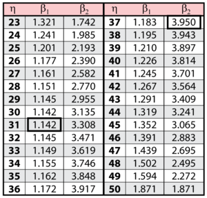
The solution is an iterative process that requires setting the value of [math]\displaystyle{ \beta\,\! }[/math] and finding the appropriate values of [math]\displaystyle{ \eta\,\! }[/math], and vice versa. The following table gives values of [math]\displaystyle{ \beta\,\! }[/math] based on given values of [math]\displaystyle{ \eta\,\! }[/math].
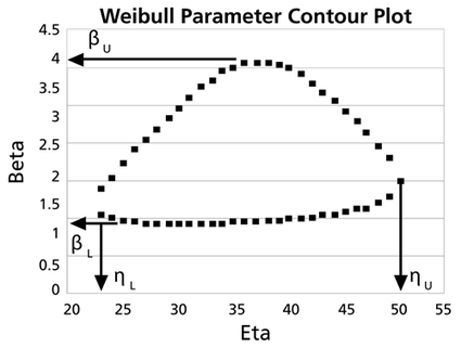
These data are represented graphically in the following contour plot:
(Note that this plot is generated with degrees of freedom [math]\displaystyle{ k = 1\,\! }[/math], as we are only determining bounds on one parameter. The contour plots generated in Weibull++ are done with degrees of freedom [math]\displaystyle{ k = 2\,\! }[/math], for use in comparing both parameters simultaneously.) As can be determined from the table, the lowest calculated value for [math]\displaystyle{ \beta\,\! }[/math] is 1.142, while the highest is 3.950. These represent the two-sided 90% confidence limits on this parameter. Since solutions for the equation do not exist for values of [math]\displaystyle{ \eta\,\! }[/math] below 23 or above 50, these can be considered the 90% confidence limits for this parameter. In order to obtain more accurate values for the confidence limits on [math]\displaystyle{ \eta\,\! }[/math], we can perform the same procedure as before, but finding the two values of [math]\displaystyle{ \eta\,\! }[/math] that correspond with a given value of [math]\displaystyle{ \beta\,\! }[/math] Using this method, we find that the 90% confidence limits on [math]\displaystyle{ \eta\,\! }[/math] are 22.474 and 49.967, which are close to the initial estimates of 23 and 50.
Note that the points where [math]\displaystyle{ \beta\,\! }[/math] are maximized and minimized do not necessarily correspond with the points where [math]\displaystyle{ \eta\,\! }[/math] are maximized and minimized. This is due to the fact that the contour plot is not symmetrical, so that the parameters will have their extremes at different points.

