Distributions Used in Accelerated Testing: Difference between revisions
| Line 164: | Line 164: | ||
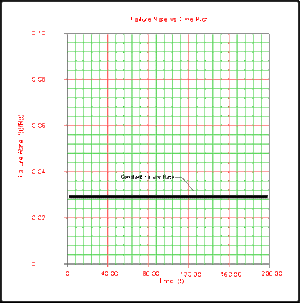
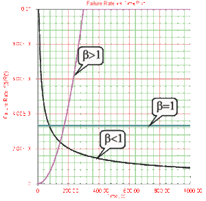
The failure rate function for the exponential distribution is constant and it is equal to the parameter <math>\lambda </math> . | The failure rate function for the exponential distribution is constant and it is equal to the parameter <math>\lambda </math> . | ||
<br> | <br> | ||
[[Image:ALTA4FRvsTP.gif|thumb|center| | [[Image:ALTA4FRvsTP.gif|thumb|center|300px|Failure Rate plot of the exponential distribution.]] | ||
<br> | <br> | ||
Revision as of 21:04, 16 August 2011
Life Distributions
In this section we will briefly present three lifetime distributions commonly used in accelerated
life test analysis, namely the 1-parameter exponential, the 2-parameter Weibull and the lognormal
distributions. Readers who are interested in a more rigorous overview or in different forms of
these and other life distributions can refer to ReliaSoft's Life Data Analysis Reference, Chapters 6-10 [31].
The Exponential Distribution
The exponential distribution is a very commonly used distribution in reliability engineering. Due to its simplicity, it has been widely employed even in cases to which it does not apply. The exponential distribution is used to describe units that have a constant failure rate.
The single-parameter exponential [math]\displaystyle{ pdf }[/math] is given by:
- [math]\displaystyle{ \begin{align} & f(T)= & \lambda {{e}^{-\lambda T}}=\frac{1}{m}{{e}^{-\tfrac{1}{m}T}} \\ & T\ge & 0,\lambda \gt 0,m\gt 0 \end{align} }[/math]
where:
• [math]\displaystyle{ \lambda = }[/math] constant failure rate, in failures per unit of measurement, e.g. failures per hour, per cycle, etc.
• [math]\displaystyle{ \lambda =\tfrac{1}{m}. }[/math]
• [math]\displaystyle{ m= }[/math] mean time between failures, or to a failure.
• [math]\displaystyle{ T= }[/math] operating time, life, or age, in hours, cycles, miles, actuations, etc.
This distribution requires the estimation of only one parameter, [math]\displaystyle{ \lambda }[/math] , for its application.
Statistical Properties Summary
The Mean or MTTF
The mean, [math]\displaystyle{ \overline{T}, }[/math] or Mean Time To Failure (MTTF) of the 1-parameter exponential distribution is given by:
- [math]\displaystyle{ \begin{align} & \overline{T}= & \mathop{}_{0}^{\infty }t\cdot f(t)dt=\mathop{}_{0}^{\infty }t\cdot \lambda \cdot {{e}^{-\lambda t}}dt \\ & = & \frac{1}{\lambda } \end{align} }[/math]
The Median
The median, [math]\displaystyle{ \breve{T} }[/math],
of the 1-parameter exponential distribution is given by:
- [math]\displaystyle{ \breve{T}=\frac{1}{\lambda }0.693 }[/math]
The Mode
The mode, [math]\displaystyle{ \tilde{T}, }[/math]
of the 1-parameter exponential distribution is given by:
- [math]\displaystyle{ \tilde{T}=0 }[/math]
The Standard Deviation
The standard deviation, [math]\displaystyle{ {{\sigma }_{T}} }[/math] , of the 1-parameter exponential distribution is given by:
- [math]\displaystyle{ {{\sigma }_{T}}=\frac{1}{\lambda }=m }[/math]
The Reliability Function
The 1-parameter exponential reliability function is given by:
- [math]\displaystyle{ R(T)={{e}^{-\lambda T}}={{e}^{-\tfrac{T}{m}}} }[/math]
This function is the complement of the exponential cumulative distribution function or:
- [math]\displaystyle{ R(T)=1-Q(T)=1-\mathop{}_{0}^{T}f(T)dT }[/math]
and:
- [math]\displaystyle{ R(T)=1-\mathop{}_{0}^{T}\lambda {{e}^{-\lambda T}}dT={{e}^{-\lambda T}} }[/math]
Conditional Reliability
The conditional reliability function for the 1-parameter exponential distribution is given by:
- [math]\displaystyle{ R(T,t)=\frac{R(T+t)}{R(T)}=\frac{{{e}^{-\lambda (T+t)}}}{{{e}^{-\lambda T}}}={{e}^{-\lambda t}} }[/math]
which says that the reliability for a mission of [math]\displaystyle{ t }[/math] duration undertaken after the component or equipment has already accumulated [math]\displaystyle{ T }[/math] hours of operation from age zero is only a function of the mission duration, and not a function of the age at the beginning of the mission. This is referred to as the ``memoryless property.
Reliable Life
The reliable life, or the mission duration for a desired reliability goal, [math]\displaystyle{ {{t}_{R}} }[/math] , for the 1-parameter exponential distribution is given by:
- [math]\displaystyle{ \begin{align} & R({{t}_{R}})= & {{e}^{-\lambda {{t}_{R}}}} \\ & & \\ & \ln [R({{t}_{R}})]= & -\lambda {{t}_{R}} \end{align} }[/math]
or:
- [math]\displaystyle{ {{t}_{R}}=-\frac{\ln [R({{t}_{R}})]}{\lambda } }[/math]
Failure Rate Function
The exponential failure rate function is given by:
- [math]\displaystyle{ \lambda (T)=\frac{f(T)}{R(T)}=\frac{\lambda {{e}^{-\lambda (T)}}}{{{e}^{-\lambda (T)}}}=\lambda =\text{Constant} }[/math]
Characteristics
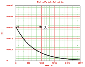
The characteristics of the 1-parameter exponential distribution can be exemplified by examining its parameter, lambda, [math]\displaystyle{ \lambda , }[/math] and the effect lambda has on the [math]\displaystyle{ pdf }[/math] , reliability and failure rate functions.
Effects of [math]\displaystyle{ \lambda }[/math] on the pdf
• The scale parameter is [math]\displaystyle{ \tfrac{1}{\lambda } }[/math] .
• As [math]\displaystyle{ \lambda }[/math] is decreased in value, the distribution is stretched out to the right, and as [math]\displaystyle{ \lambda }[/math] is increased, the distribution is pushed toward the origin.
• This distribution has no shape parameter as it has only one shape, i.e. the exponential. The only parameter it has is the failure rate, [math]\displaystyle{ \lambda }[/math] .
• The distribution starts at [math]\displaystyle{ T=0 }[/math] at the level of [math]\displaystyle{ f(T=0)=\lambda }[/math] and decreases thereafter exponentially and monotonically as [math]\displaystyle{ T }[/math] increases, and is convex.
• As [math]\displaystyle{ T\to \infty }[/math] , [math]\displaystyle{ f(T)\to 0 }[/math].
• This [math]\displaystyle{ pdf }[/math] can be thought of as a special case of the Weibull [math]\displaystyle{ pdf }[/math] with [math]\displaystyle{ \beta =1 }[/math] .
Effects of [math]\displaystyle{ \lambda }[/math] on the Reliability Function
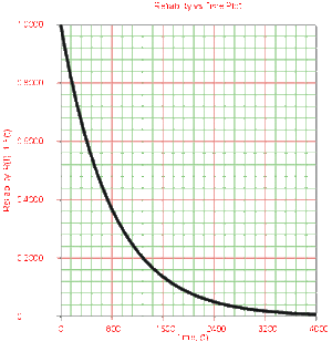
• The 1-parameter exponential reliability function starts at the value of 1 at [math]\displaystyle{ T=0 }[/math] . It decreases thereafter monotonically and is convex.
• As [math]\displaystyle{ T\to \infty }[/math] , [math]\displaystyle{ R(T\to \infty )\to 0 }[/math].
Effects of [math]\displaystyle{ \lambda }[/math] on the Failure Rate Function
The failure rate function for the exponential distribution is constant and it is equal to the parameter [math]\displaystyle{ \lambda }[/math] .
Parameter Estimation
The parameter of the exponential distribution can be estimated graphically on probability plotting paper or analytically using either least squares or maximum likelihood. (Parameter estimation methods are presented in detail in Appendix B.)
Probability Plotting
One method of calculating the parameter of the exponential distribution is by using probability plotting. To better illustrate this procedure, consider the following example.
Example 1
Let's assume six identical units are reliability tested at the same application and operation
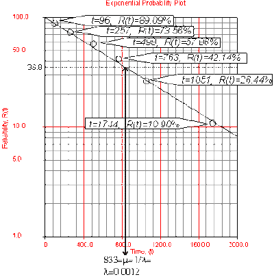
stress levels. All of these units fail during the test after operating for the following times (in hours), [math]\displaystyle{ {{T}_{i}} }[/math] : 96, 257, 498, 763, 1051 and 1744.
The steps for determining the parameters of the exponential [math]\displaystyle{ pdf }[/math] representing the
data, using probability plotting, are as follows:
• Rank the times-to-failure in ascending order as shown next.
• Obtain their median rank plotting positions.
Median rank positions are used instead of other ranking methods because median ranks are at a
specific confidence level (50%).
• The times-to-failure, with their corresponding median ranks, are shown next:
• On an exponential probability paper, plot the times on the x-axis and their corresponding
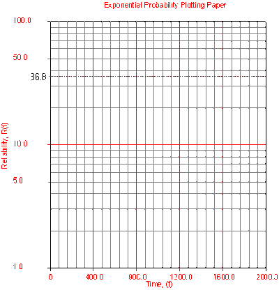
rank value on the y-axis. Fig. 4 displays an example of an exponential probability paper. The
paper is simply a log-linear paper. (The solution is given in Fig. 2.)
• Draw the best possible straight line that goes through the [math]\displaystyle{ t=0 }[/math] and [math]\displaystyle{
(t)=100% }[/math] point and through the plotted points (as shown in Fig. 5).
• At the [math]\displaystyle{ Q(t)=63.2% }[/math] or [math]\displaystyle{ R(t)=36.8% }[/math] ordinate point, draw a
straight horizontal line until this line intersects the fitted straight line. Draw a vertical line through this intersection until it crosses the abscissa. The value at the intersection of the abscissa is the estimate of the mean. For this case, [math]\displaystyle{ \widehat{\mu }=833 }[/math] hr which means that [math]\displaystyle{ \lambda =\tfrac{1}{\mu }=0.0012 }[/math] . (This is always at 63.2% since [math]\displaystyle{ (T)=1-{{e}^{-\tfrac{\mu }{\mu }}}=1-{{e}^{-1}}=0.632=63.2%). }[/math]
Now any reliability value for any mission time [math]\displaystyle{ t }[/math] can be obtained. For example, the
reliability for a mission of 15 hr, or any other time, can now be obtained either from the plot or analytically (i.e. using the equations given in Section [math]\displaystyle{ 5.1.1 }[/math] ).
To obtain the value from the plot, draw a vertical line from the abscissa, at [math]\displaystyle{ t=15 }[/math]
hr, to the fitted line. Draw a horizontal line from this intersection to the ordinate and read
[math]\displaystyle{ R(t) }[/math] . In this case, [math]\displaystyle{ R(t=15)=98.15% }[/math] . This can also be obtained
analytically, from the exponential reliability function.
MLE Parameter Estimation
The parameter of the exponential distribution can also be estimated using the maximum likelihood estimation (MLE) method. This log-likelihood function is:
- [math]\displaystyle{ \ln (L)=\Lambda =\underset{i=1}{\overset{{{F}_{e}}}{\mathop \sum }}\,{{N}_{i}}\ln \left[ \lambda {{e}^{-\lambda {{T}_{i}}}} \right]-\underset{i=1}{\overset{S}{\mathop \sum }}\,N_{i}^{\prime }\lambda T_{i}^{\prime }+\overset{FI}{\mathop{\underset{i=1}{\mathop{\underset{}{\overset{}{\mathop \sum }}\,}}\,}}\,N_{i}^{\prime \prime }\ln [R_{Li}^{\prime \prime }-R_{Ri}^{\prime \prime }] }[/math]
where:
- [math]\displaystyle{ R_{Li}^{\prime \prime }={{e}^{-\lambda T_{Li}^{\prime \prime }}} }[/math]
- [math]\displaystyle{ R_{Ri}^{\prime \prime }={{e}^{-\lambda T_{Ri}^{\prime \prime }}} }[/math]
and:
• [math]\displaystyle{ {{F}_{e}} }[/math] is the number of groups of times-to-failure data points.
• [math]\displaystyle{ {{N}_{i}} }[/math] is the number of times-to-failure in the [math]\displaystyle{ {{i}^{th}} }[/math] time-to-failure data group.
• [math]\displaystyle{ \lambda }[/math] is the failure rate parameter (unknown a priori, the only parameter to be found).
• [math]\displaystyle{ {{T}_{i}} }[/math] is the time of the [math]\displaystyle{ {{i}^{th}} }[/math] group of time-to-failure data.
• [math]\displaystyle{ S }[/math] is the number of groups of suspension data points.
• [math]\displaystyle{ N_{i}^{\prime } }[/math] is the number of suspensions in the [math]\displaystyle{ {{i}^{th}} }[/math] group of suspension data points.
• [math]\displaystyle{ T_{i}^{\prime } }[/math] is the time of the [math]\displaystyle{ {{i}^{th}} }[/math] suspension data group.
• [math]\displaystyle{ FI }[/math] is the number of interval data groups.
• [math]\displaystyle{ N_{i}^{\prime \prime } }[/math] is the number of intervals in the i [math]\displaystyle{ ^{th} }[/math] group of data intervals.
• [math]\displaystyle{ T_{Li}^{\prime \prime } }[/math] is the beginning of the i [math]\displaystyle{ ^{th} }[/math] interval.
• [math]\displaystyle{ T_{Ri}^{\prime \prime } }[/math] is the ending of the i [math]\displaystyle{ ^{th} }[/math] interval.
The solution will be found by solving for a parameter [math]\displaystyle{ \widehat{\lambda } }[/math] so that [math]\displaystyle{ \tfrac{\partial \Lambda }{\partial \lambda }=0 }[/math] where:
- [math]\displaystyle{ \frac{\partial \Lambda }{\partial \lambda }=\underset{i=1}{\overset{{{F}_{e}}}{\mathop \sum }}\,{{N}_{i}}\left( \frac{1}{\lambda }-{{T}_{i}} \right)-\underset{i=1}{\overset{S}{\mathop \sum }}\,N_{i}^{\prime }T_{i}^{\prime }-\overset{FI}{\mathop{\underset{i=1}{\mathop{\underset{}{\overset{}{\mathop \sum }}\,}}\,}}\,N_{i}^{\prime \prime }\frac{T_{Li}^{\prime \prime }R_{Li}^{\prime \prime }-T_{Ri}^{\prime \prime }R_{Ri}^{\prime \prime }}{R_{Li}^{\prime \prime }-R_{Ri}^{\prime \prime }} }[/math]
Example 2
Using the same data as in the probability plotting example (Example 1), and assuming an exponential distribution, estimate the parameter using the MLE method.
Solution
In this example we have non-grouped data without suspensions. Thus Eqn. (exp-mle) becomes:
- [math]\displaystyle{ \frac{\partial \Lambda }{\partial \lambda }=\underset{i=1}{\overset{{{F}_{e}}}{\mathop \sum }}\,\left[ \frac{1}{\lambda }-\left( {{T}_{i}} \right) \right]=\underset{i=1}{\overset{14}{\mathop \sum }}\,\left[ \frac{1}{\lambda }-\left( {{T}_{i}} \right) \right]=0 }[/math]
Substituting the values for [math]\displaystyle{ T }[/math] we get:
- [math]\displaystyle{ \begin{align} & \frac{6}{\lambda }= & 4409,\text{ or:} \\ & \lambda = & 0.00136\text{ failure/hr} \end{align} }[/math]
The Weibull Distribution
The Weibull distribution is one of the most commonly used distributions in reliability engineering because of the many shapes it attains for various values of [math]\displaystyle{ \beta }[/math] (slope). It can therefore model a great variety of data and life characteristics [18].
The 2-parameter Weibull [math]\displaystyle{ pdf }[/math] is given by:
- [math]\displaystyle{ f(T)=\frac{\beta }{\eta }{{\left( \frac{T}{\eta } \right)}^{\beta -1}}{{e}^{-{{\left( \tfrac{T}{\eta } \right)}^{\beta }}}} }[/math]
where:
- [math]\displaystyle{ f(T)\ge 0,\text{ }T\ge 0,\text{ }\beta \gt 0,\text{ }\eta \gt 0\text{ } }[/math]
and:
• [math]\displaystyle{ \eta = }[/math] scale parameter.
• [math]\displaystyle{ \beta = }[/math] shape parameter (or slope).
Statistical Properties Summary
The Mean or MTTF
The mean, [math]\displaystyle{ \overline{T}, }[/math] of the 2-parameter Weibull [math]\displaystyle{ pdf }[/math] is given by:
- [math]\displaystyle{ \overline{T}=\eta \cdot \Gamma \left( \frac{1}{\beta }+1 \right) }[/math]
where [math]\displaystyle{ \Gamma \left( \tfrac{1}{\beta }+1 \right) }[/math] is the gamma function evaluated at the value of [math]\displaystyle{ \left( \tfrac{1}{\beta }+1 \right) }[/math] .
The Median
The median, [math]\displaystyle{ \breve{T}, }[/math]
of the 2-parameter Weibull is given by:
- [math]\displaystyle{ \breve{T}=\eta {{\left( \ln 2 \right)}^{\tfrac{1}{\beta }}} }[/math]
The Mode
The mode, [math]\displaystyle{ \tilde{T}, }[/math]
of the 2-parameter Weibull is given by:
- [math]\displaystyle{ \tilde{T}=\eta {{\left( 1-\frac{1}{\beta } \right)}^{\tfrac{1}{\beta }}} }[/math]
The Standard Deviation
The standard deviation, [math]\displaystyle{ {{\sigma }_{T}}, }[/math] of the 2-parameter Weibull is given by:
- [math]\displaystyle{ {{\sigma }_{T}}=\eta \cdot \sqrt{\Gamma \left( \frac{2}{\beta }+1 \right)-\Gamma {{\left( \frac{1}{\beta }+1 \right)}^{2}}} }[/math]
The [math]\displaystyle{ cdf }[/math] and the Reliability Function
The [math]\displaystyle{ cdf }[/math] of the 2-parameter Weibull distribution is given by:
- [math]\displaystyle{ F(T)=1-{{e}^{-{{\left( \tfrac{T}{\eta } \right)}^{\beta }}}} }[/math]
The Weibull reliability function is given by:
- [math]\displaystyle{ \begin{align} & R(T)= & 1-F(t) \\ & = & {{e}^{-{{\left( \tfrac{T}{\eta } \right)}^{\beta }}}} \end{align} }[/math]
The Conditional Reliability Function
The Weibull conditional reliability function is given by:
- [math]\displaystyle{ R(T,t)=\frac{R(T+t)}{R(T)}=\frac{{{e}^{-{{\left( \tfrac{T+t}{\eta } \right)}^{\beta }}}}}{{{e}^{-{{\left( \tfrac{T}{\eta } \right)}^{\beta }}}}} }[/math]
or:
- [math]\displaystyle{ R(T,t)={{e}^{-\left[ {{\left( \tfrac{T+t}{\eta } \right)}^{\beta }}-{{\left( \tfrac{T}{\eta } \right)}^{\beta }} \right]}} }[/math]
Eqn. (e137) gives the reliability for a new mission of [math]\displaystyle{ t }[/math] duration, having already accumulated [math]\displaystyle{ T }[/math] hours of operation up to the start of this new mission, and the units are checked out to assure that they will start the next mission successfully. (It is called conditional because you can calculate the reliability of a new mission based on the fact that the unit(s) already accumulated [math]\displaystyle{ T }[/math] hours of operation successfully.)
The Reliable Life
For the 2-parameter Weibull distribution, the reliable life, [math]\displaystyle{ {{T}_{R}} }[/math] , of a unit for a specified reliability, starting the mission at age zero, is given by:
- [math]\displaystyle{ {{T}_{R}}=\eta \cdot {{\left\{ -\ln \left[ R\left( {{T}_{R}} \right) \right] \right\}}^{\tfrac{1}{\beta }}} }[/math]
This is the life for which the unit will function successfully with a reliability of [math]\displaystyle{ R({{T}_{R}}) }[/math] . If [math]\displaystyle{ R({{T}_{R}})=0.50 }[/math] then [math]\displaystyle{ {{T}_{R}}=\breve{T} }[/math],
the median life, or the life by which half of the units will survive.
The Failure Rate Function
The 2-parameter Weibull failure rate function,[math]\displaystyle{ \lambda (T) }[/math] ,
is given by:
- [math]\displaystyle{ \lambda \left( T \right)=\frac{f\left( T \right)}{R\left( T \right)}=\frac{\beta }{\eta }{{\left( \frac{T}{\eta } \right)}^{\beta -1}} }[/math]
Characteristics
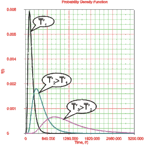
The characteristics of the 2-parameter Weibull distribution can be exemplified by examining the two parameters, beta, [math]\displaystyle{ \beta , }[/math] and eta, [math]\displaystyle{ \eta , }[/math] and the effect they have on the [math]\displaystyle{ pdf, }[/math] reliability and failure rate functions.
Looking at [math]\displaystyle{ \beta }[/math]
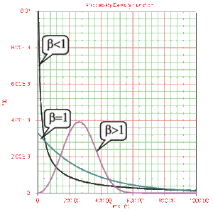
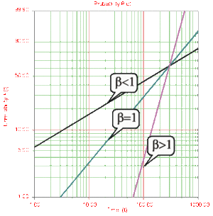
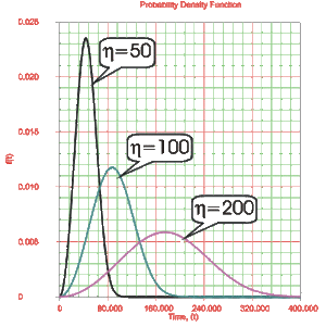
Beta, [math]\displaystyle{ \beta , }[/math] is called the shape parameter or slope of the Weibull distribution. Changing the value of [math]\displaystyle{ \beta }[/math] forces a change in the shape of the [math]\displaystyle{ pdf }[/math] as shown in Fig. 6. In addition, when the [math]\displaystyle{ cdf }[/math] is plotted on Weibull probability paper, as shown in Fig. 7, a change in beta is a change in the slope of the distribution on Weibull probability paper.
Effects of [math]\displaystyle{ \beta }[/math] on the pdf
• For [math]\displaystyle{ 0\lt \beta \lt 1 }[/math] , the failure rate decreases with time and:
- o As [math]\displaystyle{ T\to 0, }[/math] [math]\displaystyle{ f(T)\to \infty . }[/math]
- o As [math]\displaystyle{ T\to \infty }[/math] , [math]\displaystyle{ f(T)\to 0 }[/math] .
- o [math]\displaystyle{ f(T) }[/math] decreases monotonically and is convex as [math]\displaystyle{ T }[/math] increases.
- o The mode is non-existent.
• For [math]\displaystyle{ \beta =1, }[/math] it becomes the exponential distribution, as a special case,
or:
- [math]\displaystyle{ f(T)=\frac{1}{\eta }{{e}^{-\tfrac{T}{\eta }}};\text{ }\eta \gt 0,T\ge 0 }[/math]
where [math]\displaystyle{ \tfrac{1}{\eta }=\lambda = }[/math] chance, useful life, or failure rate.
• For [math]\displaystyle{ \beta \gt 1 }[/math] , [math]\displaystyle{ f(T), }[/math] the Weibull assumes wear-out type shapes (i.e. the failure rate increases with time) and:
- o [math]\displaystyle{ f(T)=0 }[/math] at [math]\displaystyle{ T=0 }[/math] .
- o [math]\displaystyle{ f(T) }[/math] increases as [math]\displaystyle{ T\to \tilde{T} }[/math] (mode) and decreases thereafter.
- o For [math]\displaystyle{ \beta =2 }[/math] it becomes the Rayleigh distribution as a special case. For [math]\displaystyle{ \beta \lt 2.6 }[/math] the Weibull [math]\displaystyle{ pdf }[/math] is positively skewed (has a right tail), for [math]\displaystyle{ 2.6\lt \beta \lt 3.7 }[/math] its coefficient of skewness approaches zero (no tail); consequently, it may approximate the normal [math]\displaystyle{ pdf }[/math] , and for [math]\displaystyle{ \beta \gt 3.7 }[/math] it is negatively skewed (left tail).
• The parameter [math]\displaystyle{ \beta }[/math] is a pure number, i.e. it is dimensionless.
Effects of [math]\displaystyle{ \beta }[/math] on the Reliability Function and the cdf
• [math]\displaystyle{ R(T) }[/math] decreases sharply and monotonically for [math]\displaystyle{ 0\lt \beta \lt 1 }[/math] , it is convex, and decreases less sharply for the same [math]\displaystyle{ \beta }[/math] .
• For [math]\displaystyle{ \beta =1 }[/math] and the same [math]\displaystyle{ \eta }[/math] , [math]\displaystyle{ R(T) }[/math] decreases monotonically but less sharply than for [math]\displaystyle{ 0\lt \beta \lt 1 }[/math] , and is convex.
• For [math]\displaystyle{ \beta \gt 1 }[/math] , [math]\displaystyle{ R(T) }[/math] decreases as [math]\displaystyle{ T }[/math] increases but less sharply than before, and as wear-out sets in, it decreases sharply and goes through an inflection point.
Effects of [math]\displaystyle{ \beta }[/math] on the Failure Rate Function
• The Weibull failure rate for [math]\displaystyle{ 0\lt \beta \lt 1 }[/math] is unbounded at [math]\displaystyle{ T=0 }[/math] . The failure rate, [math]\displaystyle{ \lambda (T), }[/math] decreases thereafter monotonically and is convex, approaching the value of zero as [math]\displaystyle{ T\to \infty }[/math] or [math]\displaystyle{ \lambda (\infty )=0 }[/math] . This behavior makes it suitable for representing the failure rate of units exhibiting early-type failures, for which the failure rate decreases with age. When such behavior is encountered, one or more of the following conclusions can be drawn:
- o Burn-in testing and/or environmental stress screening are not well implemented.
- o There are problems in the production line.
- o Inadequate quality control.
- o Packaging and transit problems.
• For [math]\displaystyle{ \beta =1 }[/math] , [math]\displaystyle{ \lambda (T) }[/math] yields a constant value of [math]\displaystyle{ \tfrac{1}{\eta } }[/math] , or:
- [math]\displaystyle{ \lambda (T)=\lambda =\frac{1}{\eta } }[/math]
This makes it suitable for representing the failure rate of chance-type failures and the useful life period failure rate of units.
• For [math]\displaystyle{ \beta \gt 1 }[/math] , [math]\displaystyle{ \lambda (T) }[/math] increases as [math]\displaystyle{ T }[/math] increases and becomes suitable for representing the failure rate of units exhibiting wear-out type failures. For [math]\displaystyle{ 1\lt \beta \lt 2 }[/math] the [math]\displaystyle{ \lambda (T) }[/math] curve is concave, consequently the failure rate increases at a decreasing rate as [math]\displaystyle{ T }[/math] increases.
• For [math]\displaystyle{ \beta =2 }[/math] , or for the Rayleigh distribution case, the failure rate function is given by:
- [math]\displaystyle{ \lambda (T)=\frac{2}{\eta }\left( \frac{T}{\eta } \right) }[/math]
hence there emerges a straight line relationship between [math]\displaystyle{ \lambda (T) }[/math] and [math]\displaystyle{ T }[/math] , starting at a value of [math]\displaystyle{ \lambda (T)=0 }[/math] at [math]\displaystyle{ T=0 }[/math] , and increasing thereafter with a slope of [math]\displaystyle{ \tfrac{2}{{{\eta }^{2}}} }[/math] . Consequently, the failure rate increases at a constant rate as [math]\displaystyle{ T }[/math] increases. Furthermore, if [math]\displaystyle{ \eta =1 }[/math] the slope becomes equal to 2, and [math]\displaystyle{ \lambda (T) }[/math] becomes a straight line which passes through the origin with a slope of 2.
• When [math]\displaystyle{ \beta \gt 2 }[/math] the [math]\displaystyle{ \lambda (T) }[/math] curve is convex, with its slope increasing as [math]\displaystyle{ T }[/math] increases. Consequently, the failure rate increases at an increasing rate as [math]\displaystyle{ T }[/math] increases, indicating wear-out life.
Looking at [math]\displaystyle{ \eta }[/math]
Eta, [math]\displaystyle{ \eta , }[/math] is called the scale parameter of the Weibull distribution. The parameter [math]\displaystyle{ \eta }[/math] has the same units as [math]\displaystyle{ T }[/math] , such as hours, miles, cycles, actuations, etc.
• A change in the scale parameter [math]\displaystyle{ \eta }[/math] has the same effect on the distribution as a change of the abscissa scale.
- o If [math]\displaystyle{ \eta }[/math] is increased while [math]\displaystyle{ \beta }[/math] is kept the same, the distribution gets stretched out to the right and its height decreases, while maintaining its shape and location.
- o If [math]\displaystyle{ \eta }[/math] is decreased while [math]\displaystyle{ \beta }[/math] is kept the same, the distribution gets pushed in toward the left (i.e. toward its beginning, or 0) and its height increases.
Parameter Estimation
The estimates of the parameters of the Weibull distribution can be found graphically on probability plotting paper, or analytically using either least squares or maximum likelihood. (Parameter estimation methods are presented in detail in Appendix B.)
Probability Plotting
One method of calculating the parameters of the Weibull distribution is by using probability plotting. To better illustrate this procedure, consider the following example [18].
Example 3
Let's assume six identical units are being reliability tested at the same application and operation stress levels. All of these units fail during the test after operating the following times (in hours), [math]\displaystyle{ {{T}_{i}} }[/math] : 93, 34, 16, 120, 53 and 75.
The steps for determining the parameters of the Weibull [math]\displaystyle{ pdf }[/math] representing the data, using probability plotting, are as follows:
• Rank the times-to-failure in ascending order as shown next.
• Obtain their median rank plotting positions. The times-to-failure, with their corresponding median ranks, are shown next.
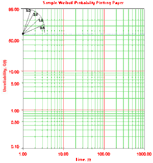
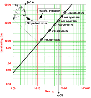
• On a Weibull probability paper, plot the times and their corresponding ranks. Fig. 11 displays an example of a Weibull probability paper (the solution is given in Fig. 12).
• Draw the best possible straight line through the plotted points (as shown in Fig. 12).
• Obtain the slope of this line by drawing a line, parallel to the one just obtained, through the slope indicator. This value is the estimate of the shape parameter [math]\displaystyle{ \widehat{\beta } }[/math] . In this case [math]\displaystyle{ \widehat{\beta }=1.4 }[/math] .
• At the [math]\displaystyle{ Q(t)=63.2% }[/math] ordinate point, draw a straight horizontal line until this line intersects the fitted straight line. Draw a vertical line through this intersection until it crosses the abscissa. The value at the intersection of the abscissa is the estimate of [math]\displaystyle{ \widehat{\eta } }[/math] . For this case [math]\displaystyle{ \widehat{\eta }=76 }[/math] hr. (This is always at 63.2% since [math]\displaystyle{ Q(T)=1-{{e}^{-{{(\tfrac{\eta }{\eta })}^{\beta }}}}=1-{{e}^{-1}}=0.632=63.2%). }[/math]
Now any reliability value for any mission time [math]\displaystyle{ t }[/math] can be obtained. For example, the reliability for a mission of 15 hr, or any other time, can now be obtained either from the plot or analytically (i.e. using the equations given in Section 5.2.1).
To obtain the value from the plot, draw a vertical line from the abscissa, at [math]\displaystyle{ t=15 }[/math] hr, to the fitted line. Draw a horizontal line from this intersection to the ordinate and read [math]\displaystyle{ Q(t) }[/math] , in this case [math]\displaystyle{ Q(t=15)=9.8% }[/math] . Thus, [math]\displaystyle{ R(t=15)=1-Q(t)=90.2% }[/math] . This can also be obtained analytically from the Weibull reliability function since both of the parameters are known.
- [math]\displaystyle{ R(t=15)={{e}^{-{{\left( \tfrac{15}{\eta } \right)}^{\beta }}}}={{e}^{-{{\left( \tfrac{15}{76} \right)}^{1.4}}}}=90.2%. }[/math]
MLE Parameter Estimation
The parameters of the 2-parameter Weibull distribution can also be estimated using Maximum Likelihood Estimation (MLE). This log-likelihood function is composed of :
- [math]\displaystyle{ \begin{align} & \ln (L)= & \Lambda =\underset{i=1}{\overset{{{F}_{e}}}{\mathop \sum }}\,{{N}_{i}}\ln \left[ \frac{\beta }{\eta }{{\left( \frac{{{T}_{i}}}{\eta } \right)}^{\beta -1}}{{e}^{-{{\left( \tfrac{{{T}_{i}}}{\eta } \right)}^{\beta }}}} \right] \\ & & -\underset{i=1}{\overset{S}{\mathop \sum }}\,N_{i}^{\prime }{{\left( \frac{T_{i}^{\prime }}{\eta } \right)}^{\beta }}\overset{FI}{\mathop{+\underset{i=1}{\mathop{\underset{}{\overset{}{\mathop \sum }}\,}}\,}}\,N_{i}^{\prime \prime }\ln [R_{Li}^{\prime \prime }-R_{Ri}^{\prime \prime }] \end{align} }[/math]
where:
- [math]\displaystyle{ R_{Li}^{\prime \prime }={{e}^{-{{(\tfrac{T_{Li}^{\prime \prime }}{\eta })}^{\beta }}}} }[/math]
- [math]\displaystyle{ R_{Ri}^{\prime \prime }={{e}^{-{{(\tfrac{T_{Ri}^{\prime \prime }}{\eta })}^{\beta }}}} }[/math]
• [math]\displaystyle{ {{F}_{e}} }[/math] is the number of groups of times-to-failure data points.
• .. is the number of times-to-failure in the [math]\displaystyle{ {{i}^{th}} }[/math] time-to-failure data group.
• [math]\displaystyle{ \beta }[/math] is the Weibull shape parameter (unknown a priori, the first of two parameters to be found).
• [math]\displaystyle{ \eta }[/math] is the Weibull scale parameter (unknown a priori, the second of two parameters to be found).
• [math]\displaystyle{ {{T}_{i}} }[/math] is the time of the [math]\displaystyle{ {{i}^{th}} }[/math] group of time-to-failure data.
• [math]\displaystyle{ S }[/math] is the number of groups of suspension data points.
• [math]\displaystyle{ N_{i}^{\prime } }[/math] is the number of suspensions in [math]\displaystyle{ {{i}^{th}} }[/math] group of suspension data points.
• [math]\displaystyle{ T_{i}^{\prime } }[/math] is the time of the [math]\displaystyle{ {{i}^{th}} }[/math] suspension data group.
• [math]\displaystyle{ FI }[/math] is the number of interval data groups.
• [math]\displaystyle{ N_{i}^{\prime \prime } }[/math] is the number of intervals in the i [math]\displaystyle{ ^{th} }[/math] group of data intervals.
• [math]\displaystyle{ T_{Li}^{\prime \prime } }[/math] is the beginning of the i [math]\displaystyle{ ^{th} }[/math] interval.
• [math]\displaystyle{ T_{Ri}^{\prime \prime } }[/math] is the ending of the i [math]\displaystyle{ ^{th} }[/math] interval.
The solution is found by solving for a pair of parameters [math]\displaystyle{ \left( \widehat{\beta },\widehat{\eta } \right) }[/math] so that [math]\displaystyle{ \tfrac{\partial \Lambda }{\partial \beta }=0 }[/math] and [math]\displaystyle{ \tfrac{\partial \Lambda }{\partial \eta }=0. }[/math] (Other methods can also be used, such as direct maximization of the likelihood function, without having to compute the derivatives.)
- [math]\displaystyle{ \begin{align} & \frac{\partial \Lambda }{\partial \beta }= & \frac{1}{\beta }\underset{i=1}{\overset{{{F}_{e}}}{\mathop{\sum }}}\,{{N}_{i}}+\underset{i=1}{\overset{{{F}_{e}}}{\mathop{\sum }}}\,{{N}_{i}}\ln \left( \frac{{{T}_{i}}}{\eta } \right) \\ & & -\underset{i=1}{\overset{{{F}_{e}}}{\mathop{\sum }}}\,{{N}_{i}}{{\left( \frac{{{T}_{i}}}{\eta } \right)}^{\beta }}\ln \left( \frac{{{T}_{i}}}{\eta } \right)-\underset{i=1}{\overset{S}{\mathop{\sum }}}\,N_{i}^{\prime }{{\left( \frac{T_{i}^{\prime }}{\eta } \right)}^{\beta }}\ln \left( \frac{T_{i}^{\prime }}{\eta } \right) \\ & & +\overset{FI}{\mathop{\underset{i=1}{\mathop{\underset{}{\overset{}{\mathop \sum }}\,}}\,}}\,N_{i}^{\prime \prime }\frac{-{{(\tfrac{T_{Li}^{\prime \prime }}{\eta })}^{\beta }}\ln (\tfrac{T_{Li}^{\prime \prime }}{\eta })R_{Li}^{\prime \prime }+{{(\tfrac{T_{Ri}^{\prime \prime }}{\eta })}^{\beta }}\ln (\tfrac{T_{Ri}^{\prime \prime }}{\eta })R_{Ri}^{\prime \prime }}{R_{Li}^{\prime \prime }-R_{Ri}^{\prime \prime }} \\ & & \\ & \frac{\partial \Lambda }{\partial \eta }= & \frac{-\beta }{\eta }\underset{i=1}{\overset{{{F}_{e}}}{\mathop{\sum }}}\,{{N}_{i}}+\frac{\beta }{\eta }\underset{i=1}{\overset{{{F}_{e}}}{\mathop{\sum }}}\,{{N}_{i}}{{\left( \frac{{{T}_{i}}}{\eta } \right)}^{\beta }} \\ & & +\frac{\beta }{\eta }\underset{i=1}{\overset{S}{\mathop{\sum }}}\,N_{i}^{\prime }{{\left( \frac{T_{i}^{\prime }}{\eta } \right)}^{\beta }}+\overset{FI}{\mathop{\underset{i=1}{\mathop{\underset{}{\overset{}{\mathop \sum }}\,}}\,}}\,N_{i}^{\prime \prime }\frac{\beta }{\eta }\frac{{{(\tfrac{T_{Li}^{\prime \prime }}{\eta })}^{\beta }}R_{Li}^{\prime \prime }-{{(\tfrac{T_{Ri}^{\prime \prime }}{\eta })}^{\beta }}R_{Ri}^{\prime \prime }}{R_{Li}^{\prime \prime }-R_{Ri}^{\prime \prime }}. \end{align} }[/math]
Example 4
Using the same data as in the probability plotting example (Example 3), and assuming a 2-parameter Weibull distribution, estimate the parameter using the MLE method.
Solution
In this case we have non-grouped data with no suspensions, thus Eqns. (mle2w1) and (mle2w2) become:
- [math]\displaystyle{ \frac{\partial \Lambda }{\partial \beta }=\frac{6}{\beta }+\underset{i=1}{\overset{6}{\mathop{\sum }}}\,\ln \left( \frac{{{T}_{i}}}{\eta } \right)-\underset{i=1}{\overset{6}{\mathop{\sum }}}\,{{\left( \frac{{{T}_{i}}}{\eta } \right)}^{\beta }}\ln \left( \frac{{{T}_{i}}}{\eta } \right)=0 }[/math]
and:
- [math]\displaystyle{ \frac{\partial \Lambda }{\partial \eta }=\frac{-\beta }{\eta }\cdot 6+\frac{\beta }{\eta }\underset{i=1}{\overset{6}{\mathop \sum }}\,{{\left( \frac{{{T}_{i}}}{\eta } \right)}^{\beta }}=0 }[/math]
Solving the above equations simultaneously we get:
- [math]\displaystyle{ \begin{matrix} \widehat{\beta }=1.933 \\ \widehat{\eta }=73.526 \\ \end{matrix} }[/math]
The Lognormal Distribution
The lognormal distribution is commonly used for general reliability analysis, cycles-to-failure in fatigue, material strengths and loading variables in probabilistic design. A random variable is lognormally distributed if the logarithm of the random variable is normally distributed. Since the logarithms of a lognormally distributed random variable are normally distributed, the lognormal distribution is given by:
- [math]\displaystyle{ f({T}')=\frac{1}{{{\sigma }_{{{T}'}}}\sqrt{2\pi }}{{e}^{-\tfrac{1}{2}{{\left( \tfrac{{T}'-\bar{{T}'}}{{{\sigma }_{{{T}'}}}} \right)}^{2}}}} }[/math]
where:
• [math]\displaystyle{ {T}'=\ln T }[/math] , and where the [math]\displaystyle{ T }[/math] s are the times-to-failure.
• [math]\displaystyle{ \bar{{T}'}= }[/math] mean of the natural logarithms of the times to failure.
• [math]\displaystyle{ {{\sigma }_{{{T}'}}}= }[/math] standard deviation of the natural logarithms of the times to failure.
The lognormal [math]\displaystyle{ pdf }[/math] can be obtained, realizing that for equal probabilities under the normal and lognormal [math]\displaystyle{ pdf }[/math] s incremental areas should also be equal, or:
- [math]\displaystyle{ f(T)dT=f({T}')d{T}' }[/math]
Taking the derivative yields:
- [math]\displaystyle{ d{T}'=\frac{dT}{T} }[/math]
Substitution yields:
- [math]\displaystyle{ \begin{align} & f(T)= & \frac{f({T}')}{T} \\ & = & \frac{1}{T\cdot {{\sigma }_{{{T}'}}}\sqrt{2\pi }}{{e}^{-\tfrac{1}{2}{{\left( \tfrac{{T}'-\bar{{T}'}}{{{\sigma }_{{{T}'}}}} \right)}^{2}}}} \end{align} }[/math]
where:
- [math]\displaystyle{ f(T)\ge 0,T\gt 0,-\infty \lt \bar{{T}'}\lt \infty ,{{\sigma }_{{{T}'}}}\gt 0 }[/math]
Statistical Properties Summary
The Mean or MTTF
• The mean of the lognormal distribution, [math]\displaystyle{ \bar{T} }[/math] , is given by:
- [math]\displaystyle{ \bar{T}={{e}^{\bar{{T}'}+\tfrac{1}{2}\sigma _{{{T}'}}^{2}}} }[/math]
• The mean of the natural logarithms of the times-to-failure, [math]\displaystyle{ {{\bar{T}}^{^{\prime }}} }[/math] , in terms of [math]\displaystyle{ \bar{T} }[/math] and [math]\displaystyle{ {{\sigma }_{T}} }[/math] is given by:
- [math]\displaystyle{ {{\bar{T}}^{\prime }}=\ln \left( {\bar{T}} \right)-\frac{1}{2}\ln \left( \frac{\sigma _{T}^{2}}{{{{\bar{T}}}^{2}}}+1 \right) }[/math]
The Standard Deviation
• The standard deviation of the lognormal distribution, [math]\displaystyle{ {{\sigma }_{T}} }[/math] , is given by:
- [math]\displaystyle{ {{\sigma }_{T}}=\sqrt{\left( {{e}^{2\bar{{T}'}+\sigma _{{{T}'}}^{2}}} \right)\left( {{e}^{\sigma _{{{T}'}}^{2}}}-1 \right)} }[/math]
• The standard deviation of the natural logarithms of the times-to-failure, [math]\displaystyle{ {{\sigma }_{{{T}'}}} }[/math] , in terms of [math]\displaystyle{ \bar{T} }[/math] and [math]\displaystyle{ {{\sigma }_{T}} }[/math] is given by:
- [math]\displaystyle{ {{\sigma }_{{{T}'}}}=\sqrt{\ln \left( \frac{\sigma _{T}^{2}}{{{{\bar{T}}}^{2}}}+1 \right)} }[/math]
The Median
• The median of the lognormal distribution is given by:
- [math]\displaystyle{ \breve{T}={{e}^{{{\bar{T}}^{\prime }}}} }[/math]
The Mode
• The mode of the lognormal distribution is given by:
- [math]\displaystyle{ \tilde{T}={{e}^{{{\bar{T}}^{\prime }}-\sigma _{{{T}'}}^{2}}} }[/math]
Reliability Function
For the lognormal distribution, the reliability for a mission of time [math]\displaystyle{ T }[/math] , starting at age 0, is given by:
- [math]\displaystyle{ R(T)=\mathop{}_{T}^{\infty }f(t)dt }[/math]
or:
- [math]\displaystyle{ R(T)=\mathop{}_{{{T}^{^{\prime }}}}^{\infty }\frac{1}{{{\sigma }_{{{T}'}}}\sqrt{2\pi }}{{e}^{-\tfrac{1}{2}{{\left( \tfrac{t-\overline{{{T}'}}}{{{\sigma }_{{{T}'}}}} \right)}^{2}}}}dt }[/math]
There is no closed form solution for the lognormal reliability function. Solutions can be obtained via the use of standard normal tables.
Lognormal Failure Rate
The lognormal failure rate is given by:
- [math]\displaystyle{ \lambda (T)=\frac{f(T)}{R(T)}=\frac{\tfrac{1}{{T}'{{\sigma }_{{{T}'}}}\sqrt{2\pi }}{{e}^{-\tfrac{1}{2}{{(\tfrac{{T}'-\overline{{{T}'}}}{{{\sigma }_{{{T}'}}}})}^{2}}}}}{\mathop{}_{{{T}'}}^{\infty }\tfrac{1}{{{\sigma }_{{{T}'}}}\sqrt{2\pi }}{{e}^{-\tfrac{1}{2}{{(\tfrac{t-\overline{{{T}'}}}{{{\sigma }_{{{T}'}}}})}^{2}}}}dt} }[/math]
Characteristics
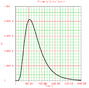
• The lognormal distribution is a distribution skewed to the right.
• The [math]\displaystyle{ pdf }[/math] starts at zero, increases to its mode, and decreases thereafter.
The characteristics of the lognormal distribution can be exemplified by examining the two parameters, the log-mean, [math]\displaystyle{ ({{\overline{T}}^{\prime }}), }[/math] and the log-std, [math]\displaystyle{ ({{\sigma }_{{{T}'}}}), }[/math] and the effect they have on the [math]\displaystyle{ pdf }[/math] .
Looking at the Log-Mean [math]\displaystyle{ ({{\overline{T}}^{\prime }}) }[/math]
• The parameter, [math]\displaystyle{ \bar{{T}'} }[/math] , or the log-mean life, or the [math]\displaystyle{ MTT{F}' }[/math] in terms of the logarithm of the [math]\displaystyle{ {T}'s }[/math] is also the scale parameter, and is a unitless number.
• For the same [math]\displaystyle{ {{\sigma }_{{{T}'}}} }[/math] the [math]\displaystyle{ pdf }[/math] 's skewness increases as [math]\displaystyle{ \bar{{T}'} }[/math] increases.
Looking at the Log-STD [math]\displaystyle{ ({{\sigma }_{{{T}'}}}) }[/math]
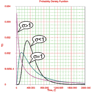
• The parameter [math]\displaystyle{ {{\sigma }_{{{T}'}}} }[/math] , or the standard deviation of the [math]\displaystyle{ {T}'s }[/math] in terms of their logarithm or of their [math]\displaystyle{ {T}' }[/math] , is also the shape parameter, and not the scale parameter as in the normal [math]\displaystyle{ pdf }[/math] . It is a unitless number and assumes only positive values.
• The degree of skewness increases as [math]\displaystyle{ {{\sigma }_{{{T}'}}} }[/math] increases, for a given [math]\displaystyle{ \bar{{T}'} }[/math] .
• For [math]\displaystyle{ {{\sigma }_{{{T}'}}} }[/math] values significantly greater than 1, the [math]\displaystyle{ pdf }[/math] rises very sharply in the beginning (i.e. for very small values of [math]\displaystyle{ T }[/math] near zero), and essentially follows the ordinate axis, peaks out early, and then decreases sharply like an exponential [math]\displaystyle{ pdf }[/math] or a Weibull [math]\displaystyle{ pdf }[/math] with [math]\displaystyle{ 0\lt \beta \lt 1 }[/math] .
Parameter Estimation
The estimate of the parameters of the lognormal distribution can be found graphically on probability plotting paper or analytically using either least squares or maximum likelihood. (Parameter estimation methods are presented in detail in Appendix B.)
Probability Plotting
One method of calculating the parameter of the lognormal distribution is by using probability plotting. To better illustrate this procedure, consider the following example.
Example 5
Let's assume six identical units are being reliability tested at the same application and operation stress levels. All of these units fail during the test after operating the following times (in hours), [math]\displaystyle{ {{T}_{i}} }[/math] : 144, 385, 747, 1,144, 1,576 and 2,616.
The steps for determining the parameters of the lognormal [math]\displaystyle{ pdf }[/math] representing the data, using probability plotting, are as follows:
• Rank the times-to-failure in ascending order as shown next.
• Obtain their median rank plotting positions. The times-to-failure, with their corresponding median ranks, are shown next:
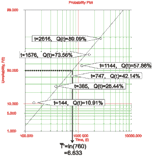
• On a lognormal probability paper, plot the times and their corresponding rank value. Fig. 16 displays an example of a lognormal probability paper. The paper is simply a log-log paper. (The solution is given in Fig. 17.)
• Draw the best possible straight line that goes through the [math]\displaystyle{ t=0 }[/math]
and [math]\displaystyle{ R(t)=100% }[/math] point and through these points (as shown in Fig. 17).
• At the [math]\displaystyle{ Q(t)=50% }[/math] ordinate point, draw a straight horizontal line until this line intersects the fitted straight line. Draw a vertical line through this intersection until it crosses the abscissa. The value at the intersection of the abscissa is the estimate of the median. For this case, [math]\displaystyle{ \breve{T}=760 }[/math] hr which means that [math]\displaystyle{ {{\bar{T}}^{\prime }}=\ln(\breve{T})=6.633 }[/math](see Eqn. Median).
- [math]\displaystyle{ }[/math]
• The standard deviation, [math]\displaystyle{ {{\sigma }_{{{T}'}}}, }[/math] can be found using the following equation:
- [math]\displaystyle{ \begin{align} & {{\sigma }_{{{T}'}}}= & \frac{\ln \left[ T(Q=97.7%) \right]-\ln \left[ T(Q=2.3%) \right]}{4} \\ & = & \frac{\ln (5100)-\ln (120)}{4} \\ & = & 0.937376 \end{align} }[/math]
Now any reliability value for any mission time [math]\displaystyle{ t }[/math] can be obtained. For example, the reliability for a mission of 200 hr, or any other time, can now be obtained either from the plot or analytically.
To obtain the value from the plot, draw a vertical line from the abscissa, at [math]\displaystyle{ t=200 }[/math] hr, to the fitted line. Draw a horizontal line from this intersection to the ordinate and read [math]\displaystyle{ Q(t) }[/math] . In this case, [math]\displaystyle{ R(t=200)=1-Q(t=200)=92% }[/math] . This can also be obtained analytically, from the lognormal reliability function. However, standard normal tables (or the Quick Statistical Reference in ALTA) must be used.
MLE Parameter Estimation
The parameters of the lognormal distribution can also be estimated using Maximum Likelihood Estimation (MLE). This general log-likelihood function is:
- [math]\displaystyle{ \begin{align} & \ln (L)= & \Lambda =\underset{i=1}{\overset{{{F}_{e}}}{\mathop \sum }}\,{{N}_{i}}\ln \left[ \frac{1}{{{\sigma }_{{{T}'}}}{{T}_{i}}}\phi \left( \frac{\ln \left( {{T}_{i}} \right)-{\mu }'}{{{\sigma }_{{{T}'}}}} \right) \right] \\ & & \text{ }+\underset{i=1}{\overset{S}{\mathop \sum }}\,N_{i}^{\prime }\ln \left[ 1-\Phi \left( \frac{\ln \left( T_{i}^{\prime } \right)-{\mu }'}{{{\sigma }_{{{T}'}}}} \right) \right]+\overset{FI}{\mathop{\underset{i=1}{\mathop{\underset{}{\overset{}{\mathop \sum }}\,}}\,}}\,N_{i}^{\prime \prime }\ln [\Phi (z_{Ri}^{\prime \prime })-\Phi (z_{Li}^{\prime \prime })] \end{align} }[/math]
where:
- [math]\displaystyle{ z_{Li}^{\prime \prime }=\frac{\ln T_{Li}^{\prime \prime }-{\mu }'}{\sigma _{T}^{\prime }} }[/math]
- [math]\displaystyle{ z_{Ri}^{\prime \prime }=\frac{\ln T_{Ri}^{\prime \prime }-{\mu }'}{\sigma _{T}^{\prime }} }[/math]
and:
• [math]\displaystyle{ {{F}_{e}} }[/math] is the number of groups of times-to-failure data points.
• [math]\displaystyle{ {{N}_{i}} }[/math] is the number of times-to-failure in the [math]\displaystyle{ {{i}^{th}} }[/math] time-to-failure data group.
• [math]\displaystyle{ {\mu }' }[/math] is the mean of the natural logarithms of the times-to-failure (unknown a priori, the first of two parameters to be found).
• [math]\displaystyle{ {{\sigma }_{{{T}'}}} }[/math] is the standard deviation of the natural logarithms of the times-to-failure (unknown a priori, the second of two parameters to be found).
• [math]\displaystyle{ {{T}_{i}} }[/math] is the time of the [math]\displaystyle{ {{i}^{th}} }[/math] group of time-to-failure data.
• [math]\displaystyle{ S }[/math] is the number of groups of suspension data points.
• [math]\displaystyle{ N_{i}^{\prime } }[/math] is the number of suspensions in [math]\displaystyle{ {{i}^{th}} }[/math] group of suspension data points.
• [math]\displaystyle{ T_{i}^{\prime } }[/math] is the time of the [math]\displaystyle{ {{i}^{th}} }[/math] suspension data group.
• [math]\displaystyle{ FI }[/math] is the number of interval data groups.
• [math]\displaystyle{ N_{i}^{\prime \prime } }[/math] is the number of intervals in the i [math]\displaystyle{ ^{th} }[/math] group of data intervals.
• [math]\displaystyle{ T_{Li}^{\prime \prime } }[/math] is the beginning of the i [math]\displaystyle{ ^{th} }[/math] interval.
• [math]\displaystyle{ T_{Ri}^{\prime \prime } }[/math] is the ending of the i [math]\displaystyle{ ^{th} }[/math] interval.
The solution will be found by solving for a pair of parameters [math]\displaystyle{ \left( {\mu }',{{\sigma }_{{{T}'}}} \right) }[/math] so that [math]\displaystyle{ \tfrac{\partial \Lambda }{\partial {\mu }'}=0 }[/math] and [math]\displaystyle{ \tfrac{\partial \Lambda }{\partial {{\sigma }_{{{T}'}}}}=0, }[/math] where:
- [math]\displaystyle{ \begin{align} & \frac{\partial \Lambda }{\partial {\mu }'}= & \frac{1}{\sigma _{{{T}'}}^{2}}\underset{i=1}{\overset{{{F}_{e}}}{\mathop \sum }}\,{{N}_{i}}(\ln ({{T}_{i}})-{\mu }') \\ & & +\frac{1}{{{\sigma }_{{{T}'}}}}\underset{i=1}{\overset{S}{\mathop \sum }}\,N_{i}^{\prime }\frac{\phi \left( \tfrac{\ln \left( T_{i}^{\prime } \right)-{\mu }'}{{{\sigma }_{{{T}'}}}} \right)}{1-\Phi \left( \tfrac{\ln \left( T_{i}^{\prime } \right)-{\mu }'}{{{\sigma }_{{{T}'}}}} \right)}\overset{FI}{\mathop{\underset{i=1}{\mathop{-\underset{}{\overset{}{\mathop \sum }}\,}}\,}}\,N_{i}^{\prime \prime }\frac{\varphi (z_{Ri}^{\prime \prime })-\varphi (z_{Li}^{\prime \prime })}{\sigma _{T}^{\prime }(\Phi (z_{Ri}^{\prime \prime })-\Phi (z_{Li}^{\prime \prime }))} \\ & & \\ & \frac{\partial \Lambda }{\partial {{\sigma }_{{{T}'}}}}= & \underset{i=1}{\overset{{{F}_{e}}}{\mathop \sum }}\,{{N}_{i}}\left( \frac{{{\left( \ln ({{T}_{i}})-{\mu }' \right)}^{2}}}{\sigma _{{{T}'}}^{3}}-\frac{1}{{{\sigma }_{{{T}'}}}} \right) \\ & & +\frac{1}{{{\sigma }_{{{T}'}}}}\underset{i=1}{\overset{S}{\mathop \sum }}\,N_{i}^{\prime }\frac{\left( \tfrac{\ln \left( T_{i}^{\prime } \right)-{\mu }'}{{{\sigma }_{{{T}'}}}} \right)\phi \left( \tfrac{\ln \left( T_{i}^{\prime } \right)-{\mu }'}{{{\sigma }_{{{T}'}}}} \right)}{1-\Phi \left( \tfrac{\ln \left( T_{i}^{\prime } \right)-{\mu }'}{{{\sigma }_{{{T}'}}}} \right)}\overset{FI}{\mathop{\underset{i=1}{\mathop{-\underset{}{\overset{}{\mathop \sum }}\,}}\,}}\,N_{i}^{\prime \prime }\frac{z_{Ri}^{\prime \prime }\varphi (z_{Ri}^{\prime \prime })-z_{Li}^{\prime \prime }\varphi (z_{Li}^{\prime \prime })}{\sigma _{T}^{\prime }(\Phi (z_{Ri}^{\prime \prime })-\Phi (z_{Li}^{\prime \prime }))} \end{align} }[/math]
and:
- [math]\displaystyle{ \phi \left( x \right)=\frac{1}{\sqrt{2\pi }}\cdot {{e}^{-\tfrac{1}{2}{{\left( x \right)}^{2}}}} }[/math]
- [math]\displaystyle{ \Phi (x)=\frac{1}{\sqrt{2\pi }}\mathop{}_{-\infty }^{x}{{e}^{-\tfrac{{{t}^{2}}}{2}}}dx }[/math]
Example 6
Using the same data as in the probability plotting example (Example 5), and assuming a lognormal distribution, estimate the parameters using the MLE method.
Solution
In this example we have non-grouped data without suspensions. Thus, the partials reduce to:
- [math]\displaystyle{ \begin{align} & \frac{\partial \Lambda }{\partial {\mu }'}= & \frac{1}{\sigma _{{{T}'}}^{2}}\cdot \underset{i=1}{\overset{14}{\mathop \sum }}\,\ln ({{T}_{i}})-{\mu }'=0 \\ & \frac{\partial \Lambda }{\partial {{\sigma }_{{{T}'}}}}= & \underset{i=1}{\overset{14}{\mathop \sum }}\,\left( \frac{\ln ({{T}_{i}})-{\mu }'}{\sigma _{{{T}'}}^{3}}-\frac{1}{{{\sigma }_{{{T}'}}}} \right)=0 \end{align} }[/math]
Substituting the values of [math]\displaystyle{ {{T}_{i}} }[/math] and solving the above system simultaneously, we get:
- [math]\displaystyle{ \begin{align} & {{\sigma }_{{{T}'}}}= & 0.9537 \\ & {\mu }'= & 6.6356 \end{align} }[/math]
The mean and standard deviation of the times-to-failure can be estimated using Eqns. (mean) and (sdv):
- [math]\displaystyle{ \overline{T}=\mu =1,200.31\text{ }hr }[/math]
and:
- [math]\displaystyle{ {{\sigma }_{T}}=1,461.78\text{ }hr }[/math]
| The material on this page is copyrighted. | ©1992-2012. ReliaSoft Corporation. ALL RIGHTS RESERVED. |
[[Category:Acclerated_Testing_Reference]

