Target Reliability Tool

Product reliability affects total product costs in multiple ways. Increasing product reliability increases the initial cost of producing a product but decreases other costs incurred over the life of the product. For example, increased reliability results in lower warranty and replacement costs for defective products. Increased reliability also results in greater market share as satisfied customers typically become repeat customers and recommend reliable products to others. A minimal total product cost can be determined by calculating the optimum reliability for such a product. The Target Reliability Estimator does this by minimizing the sum of lost sales costs, warranty costs and manufacturing costs.

Lost Sales Cost

The lost sales cost is caused due to lost market share. It is caused by customers choosing to go elsewhere for goods and services. The lost sales cost depends on the total market value for a product and the actual sales revenue of a product. \begin{equation} \text{Lost sales cost}=\text{Max}\{0, \text{Total Market Value}–\text{Sales Revenue}\} \end{equation} Total market value is the product of maximum market potential (number of units of product) and median market unit sale price. \begin{equation} \text{Total Market Value}=\text{Maximum Market Potential}\times\text{Median Market Unit Sale Price} \end{equation} For example, if the maximum number of units of product demanded by the market were 100,000 and the median market unit sale price was $12.00, then the total market value would be \begin{equation} 100,000\times \$12.00=\$1,200,000.00 \end{equation} Calculating sales revenue requires knowledge of market share and unit sale price. The function for market share \(f_{1}\left(x\right)\)is given by the equation \begin{equation} f_{1}\left(x\right)=1-e^{\left(-\left(\frac{x}{a}\right)^{b}\right)} \end{equation} where a and b are parameters fit to market share data. Consider the market share data given in the table below.

Reliability	Market Share
0.99	0.5
0.98	0.4
0.90	0.1

The parameters a and b can be solved for using the free-form data format in Weibull++, as shown below.

File:Reldata1.jpg

where Beta is the parameter b and Eta is the parameter a.

The function for unit sale price \(f_{3}\left(x\right)\) is given by

\begin{equation} f_{3}\left(x\right)=b\times e^{ax} \end{equation}

where a and b are parameters fit to data. Consider the data in the table below.

Reliabilty	Price/Unit
0.99	14
0.98	12
0.90	10

The parameters a and b can be determined using an Exponential function in the Degradation folio using the data in the table above as shown in the figure below.

As a function of reliability R, sales revenue is then calculated as \begin{equation} \text{Sales Revenue}\left(R\right)=\text{Total Market Value}\times\text{Market Share}\left(R\right)\times\text{Unit Price}\left(R\right) \end{equation} which can then be used to calculate the lost sales cost. \begin{equation} \text{Lost sales cost} = \text{Max}]\{0, \text{Total Market Value} – \text{Sales Revenue}\} \end{equation}

Manufacturing Cost

Manufacturing cost is a function of total market value, market share, and manufacturing cost per unit. The function \(f_{2}\left(x\right)\) for manufacturing cost per unit is given as \begin{equation} f_{2}\left(x\right)=b\times e^{\frac{a}{\left(1-x\right)}} \end{equation} where a and b are parameters fit to data. Using the substitution of variable \begin{equation} x'=\frac{1}{1-x} \end{equation} results in the equation \begin{equation} f_{2}\left(x'\right)=b\times e^{ax'} \end{equation} for which the parameters a and b can be determined using an Exponential function in the Degradation folio. Consider the data in the table below.

Reliability	Manufacturing Cost Per Unit
0.99	5
0.98	4
0.90	2

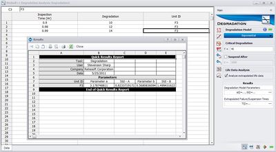
The parameters a and b can be determined using an Exponential function in the Degradation folio using the data in the table above as shown in the figure below. In the following screenshot, the “Inspection Time” column is the value of \(x'=\frac{1}{1-x}\).

File:Reldata3.jpg

Warranty Cost

Warranty cost is a function of total market value, market share, reliability, and cost per failure. The function of cost per failure \(f_{4}\left(x\right)\)is given by \begin{equation} f_{4}\left(x\right)=b\times e^{ax} \end{equation} where a and b are parameters fit to data. Consider the data below.

Reliability	Cost per Failure
0.99	3
0.98	2
0.90	1

The parameters a and b can be determined using an Exponential function in the Degradation folio using the data in the table above as shown in the figure below.

File:Reldata4.jpg

For a given reliability value R, the warranty cost is given by \begin{equation} \text{Warranty Cost}\left(R\right)=\text{Total Market Value}\times \text{Market Share}\left(R\right)\times\left(1-R\right)\times\text{Cost Per Failure}\left(R\right) \end{equation}

Total Cost

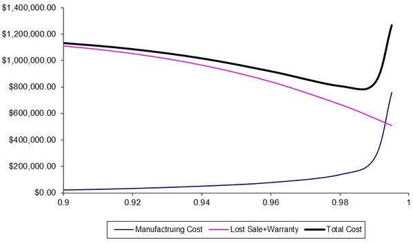
For a given reliability R, the expected total cost is given by \begin{equation} \text{Total Cost}\left(R\right) = \text{Lost Sales Cost}\left(R\right) + \text{Warranty Cost}\left(R\right) + \text{Manufacturing Cost}\left(R\right) \end{equation} The manufacturing cost is a pre-shipping cost whereas the warranty and lost sales costs are incurred after a product is shipped. These pre- and post-shipping costs can be seen in the figure below.

Note that the minimum total cost, in this example, occurs at a reliability of about 0.985.

Supplamental

	Weibull Reference Page
	This special pages additional  mathematical formulation for specific tools  in  Weibull++  8
	Weibull++

The Weibull++ Target Reliability tool

The purpose of this tool is to qualitatitivaly explore different options with regards to a target reliability for component, subsystem or system.

Inputs

There are five inputs for 3 specific cases. More specifcally:

Input Title	Input Value
Expected failures/returns per year as % of Sales	[math]\displaystyle{ Q% \text{ where } 0\le Q\le 100 \,\! }[/math]
% of market share you expect to capture	[math]\displaystyle{ S% \text{ where } 0\le S\le 100 \,\! }[/math]
Average unit sales price	[math]\displaystyle{ P \text{ where } 0\lt P \,\! }[/math]
Average cost per unit to produce	[math]\displaystyle{ C \text{ where } 0\lt C \lt P+O \,\! }[/math]
Other costs per failure	[math]\displaystyle{ O \text{ where } 0\lt O \lt C+O \,\! }[/math]

These five inputs are then repeated for three specific cases, Best Case, Most Likely and Worst Case.

Input Title	Best Case	Most Likely	Worst Case
Expected failures/returns per year as % of Sales	[math]\displaystyle{ {{Q}_{1}}\,\! }[/math]	[math]\displaystyle{ {{Q}_{2}}\,\! }[/math]	[math]\displaystyle{ {{Q}_{3}}\,\! }[/math]
% of market share you expect to capture	[math]\displaystyle{ {{S}_{1}}\,\! }[/math]	[math]\displaystyle{ {{S}_{2}}\,\! }[/math]	[math]\displaystyle{ {{S}_{3}}\,\! }[/math]
Average unit sales price	[math]\displaystyle{ {{P}_{1}}\,\! }[/math]	[math]\displaystyle{ {{P}_{2}}\,\! }[/math]	[math]\displaystyle{ {{P}_{3}}\,\! }[/math]
Average cost per unit to produce	[math]\displaystyle{ {{C}_{1}}\,\! }[/math]	[math]\displaystyle{ {{C}_{2}}\,\! }[/math]	[math]\displaystyle{ {{C}_{3}}\,\! }[/math]
Other costs per failure	[math]\displaystyle{ {{O}_{1}}\,\! }[/math]	[math]\displaystyle{ {{O}_{2}}\,\! }[/math]	[math]\displaystyle{ {{O}_{3}}\,\! }[/math]

 

  Based on the above inputs four models are then fitted as functions of reliability, [math]\displaystyle{ R=(1-Q)\,\! }[/math], or

 [math]\displaystyle{ \begin{align} & S(R)=1-{{e}^{-{{\left( \frac{R}{a} \right)}^{b}}}} \\ & P(R)=b\cdot {{e}^{\left( a\cdot R \right)}} \\ & C(R)=b\cdot {{e}^{\left( a\cdot \left( \frac{1}{1-R} \right) \right)}} \\ & F(R)=b\cdot {{e}^{\left( a\cdot R \right)}} \\ \end{align} \,\! }[/math]

 

An additional variable needed then is maximum market potential, M.

Then define and compute the following as a function of R

[math]\displaystyle{ \begin{align} &\text{Max Market Potential}=M \\ & \text{Median Sale Price}=MSP \\ & \text{Sales Revenue}=SR=M \cdot MSP \cdot S(R)\cdot P(R) \\ & \text{Warranty Cost}=WC(R)=M\cdot S(R)\cdot (1-R)\cdot F(R) \\ & \text{Manufacturing Cost}=MC(R)=M\cdot S(R)\cdot C(R) \\ & \text{Missed Sales Cost}=MSC(R)=M*MSP-Max\{0, M \cdot MSP - SR\} \\ & \text{then} \\ & \text{Production Costs}=MC(R) \\ & \text{Unreliability Costs}=WC(R)+MSC(R) \\ \end{align} \,\! }[/math]

The material on this page is copyrighted.

©1992-2012. ReliaSoft Corporation. ALL RIGHTS RESERVED.