Weibull Distribution Examples: Difference between revisions
Chris Kahn (talk | contribs) |
Lisa Hacker (talk | contribs) No edit summary |
||
| (42 intermediate revisions by 4 users not shown) | |||
| Line 1: | Line 1: | ||
<noinclude>{{Banner Weibull Examples}}{{Navigation box}} | <noinclude>{{Banner Weibull Examples}}{{Navigation box}} | ||
''These examples also appear in the [ | ''These examples also appear in the [https://help.reliasoft.com/reference/life_data_analysis Life data analysis reference].'' | ||
</noinclude> | </noinclude> | ||
===Median Rank Plot Example=== | ===Median Rank Plot Example=== | ||
In this example, we will determine the median rank value used for plotting the | In this example, we will determine the median rank value used for plotting the 6th failure from a sample size of 10. This example will use Weibull++'s Quick Statistical Reference (QSR) tool to show how the points in the plot of the following example are calculated. | ||
First, open the Quick Statistical Reference tool and select the '''Inverse F-Distribution Values''' option. | First, open the Quick Statistical Reference tool and select the '''Inverse F-Distribution Values''' option. | ||
In this example, | In this example, n1 = 10, j = 6, m = 2(10 - 6 + 1) = 10, and n2 = 2 x 6 = 12. | ||
Thus, from the F-distribution rank equation: | Thus, from the F-distribution rank equation: | ||
::<math>MR=\frac{1}{1+\left( \frac{10-6+1}{6} \right){{F}_{0.5;10;12}}}</math> | ::<math>MR=\frac{1}{1+\left( \frac{10-6+1}{6} \right){{F}_{0.5;10;12}}}\,\!</math> | ||
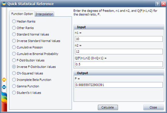
Use the QSR to calculate the value of | Use the QSR to calculate the value of F<sub>0.5;10;12</sub> = 0.9886, as shown next: | ||
[[Image: F Inverse.png|center|550px]] | [[Image: F Inverse.png|center|550px]] | ||
| Line 22: | Line 20: | ||
Consequently: | Consequently: | ||
::<math>MR=\frac{1}{1+\left( \frac{5}{6} \right)\times 0.9886}=0.5483=54.83%</math> | ::<math>MR=\frac{1}{1+\left( \frac{5}{6} \right)\times 0.9886}=0.5483=54.83%\,\!</math> | ||
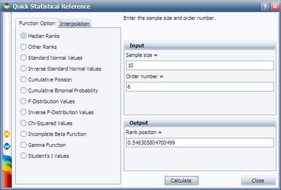
Another method is to use the '''Median Ranks''' option directly, which yields MR(%) = 54.8305%, as shown next: | Another method is to use the '''Median Ranks''' option directly, which yields MR(%) = 54.8305%, as shown next: | ||
[[Image: MR.png|center|550px]] | [[Image: MR.png|center|550px]] | ||
=== | ===Complete Data Example=== | ||
Assume that 10 identical units (N = 10) are being reliability tested at the same application and operation stress levels. 6 of these units fail during this test after operating the following numbers of hours, <math>{T}_{j}\,\!</math>: 150, 105, 83, 123, 64 and 46. The test is stopped at the 6th failure. Find the parameters of the Weibull ''pdf'' that represents these data. | |||
'''Solution''' | |||
Create a new Weibull++ standard folio that is configured for grouped times-to-failure data with suspensions. | |||
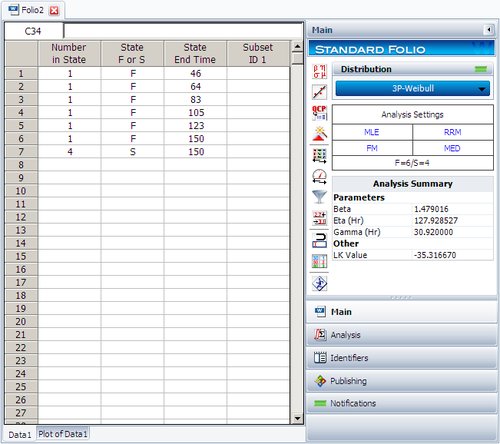
Enter the data in the appropriate columns. Note that there are 4 suspensions, as only 6 of the 10 units were tested to failure (the next figure shows the data as entered). Use the 3-parameter Weibull and MLE for the calculations. | |||
[[Image: | [[Image: DataforExample_11.png.png|center|500px]] | ||
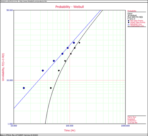
Plot the data. | |||
[[Image: Plot for Example 11.png|center|500px]] | |||
Note that the original data points, on the curved line, were adjusted by subtracting 30.92 hours to yield a straight line as shown above. | |||
===Suspension Data Example=== | |||
ACME company manufactures widgets, and it is currently engaged in reliability testing a new widget design. 19 units are being reliability tested, but due to the tremendous demand for widgets, units are removed from the test whenever the production cannot cover the demand. The test is terminated at the 67th day when the last widget is removed from the test. The following table contains the collected data. | |||
{| {| border="1" align="center" style="border-collapse: collapse;" cellpadding="5" cellspacing="5" | |||
|+ '''Widget Test Data''' | |||
| align="center" style="background:#f0f0f0;"|'''Data Point Index''' | |||
| align="center" style="background:#f0f0f0;"|'''State (F/S)''' | |||
| align="center" style="background:#f0f0f0;"|'''Time to Failure''' | |||
|- | |||
| 1||F||2 | |||
|- | |||
| 2||S||3 | |||
|- | |||
| 3||F||5 | |||
|- | |||
| 4||S||7 | |||
|- | |||
| 5||F||11 | |||
|- | |||
| 6||S||13 | |||
|- | |||
| 7||S||17 | |||
|- | |||
| 8||S||19 | |||
|- | |||
| 9||F||23 | |||
|- | |||
| 10||F||29 | |||
|- | |||
| 11||S||31 | |||
|- | |||
| 12||F||37 | |||
|- | |||
| 13||S||41 | |||
|- | |||
| 14||F||43 | |||
|- | |||
| 15||S||47 | |||
|- | |||
| 16||S||53 | |||
|- | |||
| 17||F||59 | |||
|- | |||
| 18||S||61 | |||
|- | |||
| 19||S||67 | |||
|- | |||
| | |||
|} | |||
'''Solution''' | |||
In this example, we see that the number of failures is less than the number of suspensions. This is a very common situation, since reliability tests are often terminated before all units fail due to financial or time constraints. Furthermore, some suspensions will be recorded when a failure occurs that is not due to a legitimate failure mode, such as operator error. In cases such as this, a suspension is recorded, since the unit under test cannot be said to have had a legitimate failure. | |||
Enter the data into a Weibull++ standard folio that is configured for times-to-failure data with suspensions. The folio will appear as shown next: | |||
[[Image: Data Folio Example 13.png|center|550px]] | |||
We will use the 2-parameter Weibull to solve this problem. The parameters using maximum likelihood are: | |||
::<math>\begin{align} | |||
& \hat{\beta }=1.145 \\ | |||
& \hat{\eta }=65.97 \\ | |||
\end{align}\,\!</math> | |||
Using RRX: | |||
::<math>\begin{align} | |||
& \hat{\beta }=0.914\\ | |||
& \hat{\eta }=79.38 \\ | |||
\end{align}\,\!</math> | |||
Using RRY: | |||
::<math>\begin{align} | |||
& \hat{\beta }=0.895\\ | |||
& \hat{\eta }=82.02 \\ | |||
\end{align}\,\!</math> | |||
===Interval Data Example=== | |||
Suppose we have run an experiment with 8 units tested and the following is a table of their last inspection times and failure times: | |||
{| border="1" align="center" style="border-collapse: collapse;" cellpadding="5" cellspacing="5" | |||
| align="center" style="background:#f0f0f0;"|'''Data Point Index''' | |||
| align="center" style="background:#f0f0f0;"|'''Last Inspection''' | |||
| align="center" style="background:#f0f0f0;"|'''Failure Time''' | |||
|- | |||
| 1||30||32 | |||
|- | |||
| 2||32||35 | |||
|- | |||
| 3||35||37 | |||
|- | |||
| 4||37||40 | |||
|- | |||
| 5||42||42 | |||
|- | |||
| 6||45||45 | |||
|- | |||
| 7||50||50 | |||
|- | |||
| 8||55||55 | |||
|- | |||
|} | |||
Analyze the data using several different parameter estimation techniques and compare the results. | |||
'''Solution''' | |||
Enter the data into a Weibull++ standard folio that is configured for interval data. The data is entered as follows: | |||
[[Image: Data Folio.png|center|550px]] | |||
The computed parameters using maximum likelihood are: | |||
::<math>\begin{align} | |||
& \hat{\beta }=5.76 \\ | |||
& \hat{\eta }=44.68 \\ | |||
\end{align}\,\!</math> | |||
Using RRX or rank regression on X: | |||
::<math>\begin{align} | |||
& \hat{\beta }=5.70 \\ | |||
& \hat{\eta }=44.54 \\ | |||
\end{align}\,\!</math> | |||
Using RRY or rank regression on Y: | |||
::<math>\begin{align} | |||
& \hat{\beta }=5.41 \\ | |||
& \hat{\eta }=44.76 \\ | |||
\end{align}\,\!</math> | |||
[[Image: | The plot of the MLE solution with the two-sided 90% confidence bounds is: | ||
[[Image: MLE Plot.png|center|550px]] | |||
===Mixed Data Types Example=== | |||
[[ | From Dimitri Kececioglu, Reliability & Life Testing Handbook, Page 406. [[Appendix:_Life_Data_Analysis_References|[20]]]. | ||
Estimate the parameters for the 3-parameter Weibull, for a sample of 10 units that are all tested to failure. The recorded failure times are 200; 370; 500; 620; 730; 840; 950; 1,050; 1,160 and 1,400 hours. | |||
''' | '''Published Results:''' | ||
Published results (using probability plotting): | |||
::<math>{\widehat{\beta}} = 3.0\,\!</math>, <math>{\widehat{\eta}} = 1,220\,\!</math>, <math>{\widehat{\gamma}} = -300\,\!</math> | |||
'''Computed Results in Weibull++''' | |||
Weibull++ computed parameters for rank regression on X are: | |||
::<math>{\widehat{\beta}} = 2.9013\,\!</math>, <math>{\widehat{\eta}} = 1195.5009\,\!</math>, <math>{\widehat{\gamma}} = -279.000\,\!</math> | |||
The small difference between the published results and the ones obtained from Weibull++ are due to the difference in the estimation method. In the publication the parameters were estimated using probability plotting (i.e., the fitted line was "eye-balled"). In Weibull++, the parameters were estimated using non-linear regression (a more accurate, mathematically fitted line). Note that γ in this example is negative. This means that the unadjusted for γ line is concave up, as shown next. | |||
Weibull | [[Image:Weibull Distribution Example 19 Plot.png|center|450px]] | ||
===Weibull Distribution RRX Example=== | |||
{{:Weibull_Distribution_RRX_Example}} | |||
===Benchmark with Published Examples=== | |||
The following examples compare published results to computed results obtained with Weibull++. | |||
{{Font|Complete Data RRY Example|11|Arial|bold|black}} | |||
From Dimitri Kececioglu, Reliability & Life Testing Handbook, Page 418 [[Appendix:_Life_Data_Analysis_References|[20]]]. | |||
Sample of 10 units, all tested to failure. The failures were recorded at 16, 34, 53, 75, 93, 120, 150, 191, 240 and 339 hours. | |||
'''Published Results''' | |||
Published Results (using Rank Regression on Y): | |||
::<math>\begin{align} | |||
& \widehat{\beta }=1.20 \\ | |||
& \widehat{\eta} = 146.2 \\ | |||
& \hat{\rho }=0.998703\\ | |||
\end{align}\,\!</math> | |||
'''Computed Results in Weibull++''' | '''Computed Results in Weibull++''' | ||
This same data set can be entered into a Weibull++ standard data sheet. Use RRY for the estimation method. | |||
Weibull++ computed parameters for RRY are: | |||
::<math>\begin{align} | |||
& \widehat{\beta }=1.1973 \\ | |||
& \widehat{\eta} = 146.2545 \\ | |||
& \hat{\rho }=0.9999\\ | |||
\end{align}\,\!</math> | |||
The small difference between the published results and the ones obtained from Weibull++ is due to the difference in the median rank values between the two (in the publication, median ranks are obtained from tables to 3 decimal places, whereas in Weibull++ they are calculated and carried out up to the 15th decimal point). | |||
You will also notice that in the examples that follow, a small difference may exist between the published results and the ones obtained from Weibull++. This can be attributed to the difference between the computer numerical precision employed by Weibull++ and the lower number of significant digits used by the original authors. In most of these publications, no information was given as to the numerical precision used. | |||
{{Font|Suspension Data MLE Example|11|Arial|bold|black}} | |||
From Wayne Nelson, Fan Example, Applied Life Data Analysis, page 317 [[Appendix:_Life_Data_Analysis_References|[30]]]. | |||
70 diesel engine fans accumulated 344,440 hours in service and 12 of them failed. A table of their life data is shown next (+ denotes non-failed units or suspensions, using Dr. Nelson's nomenclature). Evaluate the parameters with their two-sided 95% confidence bounds, using MLE for the 2-parameter Weibull distribution. | |||
[[Image:example18table.png|center]] | |||
'''Published Results:''' | |||
: | Weibull parameters (2P-Weibull, MLE): | ||
::<math>\begin{align} | |||
& \widehat{\beta }=1.0584 \\ | |||
& \widehat{\eta} = 26,296 \\ | |||
\end{align}\,\!</math> | |||
Published 95% FM confidence limits on the parameters: | |||
::<math>\begin{align} | |||
& \widehat{\beta }=\lbrace 0.6441, \text{ }1.7394\rbrace \\ | |||
& \widehat{\eta} = \lbrace 10,522, \text{ }65,532\rbrace \\ | |||
\end{align}\,\!</math> | |||
Published variance/covariance matrix: | |||
[[Image:example18formula3.png]] | |||
Note that Nelson expresses the results as multiples of 1,000 (or = 26.297, etc.). The published results were adjusted by this factor to correlate with Weibull++ results. | |||
'''Computed Results in Weibull++''' | |||
This same data set can be entered into a Weibull++ standard folio, using 2-parameter Weibull and MLE to calculate the parameter estimates. | |||
You can also enter the data as given in table without grouping them by opening a data sheet configured for suspension data. Then click the '''Group Data''' icon and chose '''Group exactly identical values'''. | |||
: | [[Image:groupdataicon.png|center]] | ||
[[Image:Weibull Distribution Example 18 Group Data.png|center|450px]] | |||
The data will be automatically grouped and put into a new grouped data sheet. | |||
Weibull++ computed parameters for maximum likelihood are: | |||
::<math>\begin{align} | |||
& \widehat{\beta }=1.0584 \\ | |||
& \widehat{\eta} = 26,297 \\ | |||
\end{align}\,\!</math> | |||
Weibull++ computed 95% FM confidence limits on the parameters: | |||
{{ | ::<math>\begin{align} | ||
& \widehat{\beta }=\lbrace 0.6441, \text{ }1.7394\rbrace \\ | |||
& \widehat{\eta} = \lbrace 10,522, \text{ }65,532\rbrace \\ | |||
\end{align}\,\!</math> | |||
Weibull++ computed/variance covariance matrix: | |||
[[Image:compexample18formula3.png]] | |||
''' | The two-sided 95% bounds on the parameters can be determined from the QCP. Calculate and then click '''Report''' to see the results. | ||
[[Image: Weibull Distribution Example 18 QCP Parameter Bounds.png|center|550px]] | |||
{{Font|Interval Data MLE Example|11|Arial|bold|black}} | |||
From Wayne Nelson, Applied Life Data Analysis, Page 415 [[Appendix:_Life_Data_Analysis_References|[30]]]. 167 identical parts were inspected for cracks. The following is a table of their last inspection times and times-to-failure: | |||
[[Image: | [[Image:example16table.png|center|800px]] | ||
'''Published Results:''' | |||
Published results (using MLE): | |||
== | ::<math>\begin{align} | ||
& \widehat{\beta }=1.486 \\ | |||
& \widehat{\eta} = 71.687\\ | |||
\end{align}\,\!</math> | |||
Published 95% FM confidence limits on the parameters: | |||
{ | ::<math>\begin{align} | ||
& \widehat{\beta }=\lbrace 1.224, \text{ }1.802\rbrace \\ | |||
& \widehat{\eta} = \lbrace 61.962, \text{ }82.938\rbrace \\ | |||
\end{align}\,\!</math> | |||
Published variance/covariance matrix: | |||
[[Image:example16formula3.png]] | |||
'''Computed Results in Weibull++''' | |||
This same data set can be entered into a Weibull++ standard folio that's configured for grouped times-to-failure data with suspensions and interval data. | |||
Weibull++ computed parameters for maximum likelihood are: | |||
::<math>\begin{align} | ::<math>\begin{align} | ||
& \ | & \widehat{\beta }=1.485 \\ | ||
& \widehat{\eta} = 71.690\\ | |||
\end{align}</math> | \end{align}\,\!</math> | ||
Weibull++ computed 95% FM confidence limits on the parameters: | |||
::<math>\begin{align} | ::<math>\begin{align} | ||
& \ | & \widehat{\beta }=\lbrace 1.224, \text{ }1.802\rbrace \\ | ||
& \widehat{\eta} = \lbrace 61.961, \text{ }82.947\rbrace \\ | |||
\end{align}</math> | \end{align}\,\!</math> | ||
Weibull++ computed/variance covariance matrix: | |||
: | [[Image:compexample16formula3.png]] | ||
{{Font|Grouped Suspension MLE Example|11|Arial|bold|black}} | |||
From Dallas R. Wingo, IEEE Transactions on Reliability Vol. R-22, No 2, June 1973, Pages 96-100. | |||
Wingo uses the following times-to-failure: 37, 55, 64, 72, 74, 87, 88, 89, 91, 92, 94, 95, 97, 98, 100, 101, 102, 102, 105, 105, 107, 113, 117, 120, 120, 120, 122, 124, 126, 130, 135, 138, 182. In addition, the following suspensions are used: 4 at 70, 5 at 80, 4 at 99, 3 at 121 and 1 at 150. | |||
''' | '''Published Results (using MLE)''' | ||
::<math>\begin{align} | ::<math>\begin{align} | ||
& \ | & \widehat{\beta }=3.7596935\\ | ||
& \hat{\ | & \widehat{\eta} = 106.49758 \\ | ||
\end{align}</math> | & \hat{\gamma }=14.451684\\ | ||
\end{align}\,\!</math> | |||
'''Computed Results in Weibull++''' | |||
::<math>\begin{align} | ::<math>\begin{align} | ||
& \ | & \widehat{\beta }=3.7596935\\ | ||
& \hat{\ | & \widehat{\eta} = 106.49758 \\ | ||
\end{align}</math> | & \hat{\gamma }=14.451684\\ | ||
\end{align}\,\!</math> | |||
Note that you must select the '''Use True 3-P MLE'''option in the Weibull++ Application Setup to replicate these results. | |||
{{Font|3-P Probability Plot Example|11|Arial|bold|black}} | |||
Suppose we want to model a left censored, right censored, interval, and complete data set, consisting of 274 units under test of which 185 units fail. The following | Suppose we want to model a left censored, right censored, interval, and complete data set, consisting of 274 units under test of which 185 units fail. The following table contains the data. | ||
{| {| border="1" align="center" style="border-collapse: collapse;" cellpadding="5" cellspacing="5" | {| {| border="1" align="center" style="border-collapse: collapse;" cellpadding="5" cellspacing="5" | ||
| Line 447: | Line 448: | ||
'''Solution''' | '''Solution''' | ||
Since standard ranking methods for dealing with these different data types are inadequate, we will want to use the ReliaSoft ranking method. This option is the default in Weibull++ when dealing with interval data. The filled-out standard folio is shown next: | |||
Since standard ranking methods for dealing with these different data types are inadequate, we will want to use the ReliaSoft ranking method. This option is the default in Weibull++ when dealing with interval data. The | |||
[[Image: Data Folio for Example 14.png|center|650px]] | [[Image: Data Folio for Example 14.png|center|650px]] | ||
| Line 457: | Line 454: | ||
The computed parameters using MLE are: | The computed parameters using MLE are: | ||
::<math>\hat{\beta }=0.748;\text{ }\hat{\eta }=44.38</math> | ::<math>\hat{\beta }=0.748;\text{ }\hat{\eta }=44.38\,\!</math> | ||
Using RRX: | |||
::<math>\hat{\beta }=1.057;\text{ }\hat{\eta }=36.29</math> | ::<math>\hat{\beta }=1.057;\text{ }\hat{\eta }=36.29\,\!</math> | ||
Using RRY: | |||
::<math>\hat{\beta }=0.998;\text{ }\hat{\eta }=37.16</math> | ::<math>\hat{\beta }=0.998;\text{ }\hat{\eta }=37.16\,\!</math> | ||
The plot with the two-sided 90% confidence bounds for the rank regression on X solution is: | The plot with the two-sided 90% confidence bounds for the rank regression on X solution is: | ||
[[Image: RRX Plot for Example 14.png|center|550px]] | [[Image: RRX Plot for Example 14.png|center|550px]] | ||
Latest revision as of 21:47, 18 September 2023
New format available! This reference is now available in a new format that offers faster page load, improved display for calculations and images and more targeted search.
As of January 2024, this Reliawiki page will not continue to be updated. Please update all links and bookmarks to the latest references at Weibull examples and Weibull reference examples.
These examples also appear in the Life data analysis reference.
Median Rank Plot Example
In this example, we will determine the median rank value used for plotting the 6th failure from a sample size of 10. This example will use Weibull++'s Quick Statistical Reference (QSR) tool to show how the points in the plot of the following example are calculated.
First, open the Quick Statistical Reference tool and select the Inverse F-Distribution Values option.
In this example, n1 = 10, j = 6, m = 2(10 - 6 + 1) = 10, and n2 = 2 x 6 = 12.
Thus, from the F-distribution rank equation:
- [math]\displaystyle{ MR=\frac{1}{1+\left( \frac{10-6+1}{6} \right){{F}_{0.5;10;12}}}\,\! }[/math]
Use the QSR to calculate the value of F0.5;10;12 = 0.9886, as shown next:
Consequently:
- [math]\displaystyle{ MR=\frac{1}{1+\left( \frac{5}{6} \right)\times 0.9886}=0.5483=54.83%\,\! }[/math]
Another method is to use the Median Ranks option directly, which yields MR(%) = 54.8305%, as shown next:
Complete Data Example
Assume that 10 identical units (N = 10) are being reliability tested at the same application and operation stress levels. 6 of these units fail during this test after operating the following numbers of hours, [math]\displaystyle{ {T}_{j}\,\! }[/math]: 150, 105, 83, 123, 64 and 46. The test is stopped at the 6th failure. Find the parameters of the Weibull pdf that represents these data.
Solution
Create a new Weibull++ standard folio that is configured for grouped times-to-failure data with suspensions.
Enter the data in the appropriate columns. Note that there are 4 suspensions, as only 6 of the 10 units were tested to failure (the next figure shows the data as entered). Use the 3-parameter Weibull and MLE for the calculations.
Plot the data.
Note that the original data points, on the curved line, were adjusted by subtracting 30.92 hours to yield a straight line as shown above.
Suspension Data Example
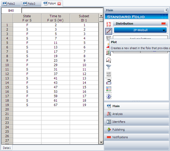
ACME company manufactures widgets, and it is currently engaged in reliability testing a new widget design. 19 units are being reliability tested, but due to the tremendous demand for widgets, units are removed from the test whenever the production cannot cover the demand. The test is terminated at the 67th day when the last widget is removed from the test. The following table contains the collected data.
| Data Point Index | State (F/S) | Time to Failure |
| 1 | F | 2 |
| 2 | S | 3 |
| 3 | F | 5 |
| 4 | S | 7 |
| 5 | F | 11 |
| 6 | S | 13 |
| 7 | S | 17 |
| 8 | S | 19 |
| 9 | F | 23 |
| 10 | F | 29 |
| 11 | S | 31 |
| 12 | F | 37 |
| 13 | S | 41 |
| 14 | F | 43 |
| 15 | S | 47 |
| 16 | S | 53 |
| 17 | F | 59 |
| 18 | S | 61 |
| 19 | S | 67 |
Solution
In this example, we see that the number of failures is less than the number of suspensions. This is a very common situation, since reliability tests are often terminated before all units fail due to financial or time constraints. Furthermore, some suspensions will be recorded when a failure occurs that is not due to a legitimate failure mode, such as operator error. In cases such as this, a suspension is recorded, since the unit under test cannot be said to have had a legitimate failure.
Enter the data into a Weibull++ standard folio that is configured for times-to-failure data with suspensions. The folio will appear as shown next:
We will use the 2-parameter Weibull to solve this problem. The parameters using maximum likelihood are:
- [math]\displaystyle{ \begin{align} & \hat{\beta }=1.145 \\ & \hat{\eta }=65.97 \\ \end{align}\,\! }[/math]
Using RRX:
- [math]\displaystyle{ \begin{align} & \hat{\beta }=0.914\\ & \hat{\eta }=79.38 \\ \end{align}\,\! }[/math]
Using RRY:
- [math]\displaystyle{ \begin{align} & \hat{\beta }=0.895\\ & \hat{\eta }=82.02 \\ \end{align}\,\! }[/math]
Interval Data Example
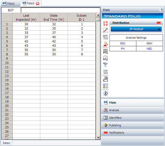
Suppose we have run an experiment with 8 units tested and the following is a table of their last inspection times and failure times:
| Data Point Index | Last Inspection | Failure Time |
| 1 | 30 | 32 |
| 2 | 32 | 35 |
| 3 | 35 | 37 |
| 4 | 37 | 40 |
| 5 | 42 | 42 |
| 6 | 45 | 45 |
| 7 | 50 | 50 |
| 8 | 55 | 55 |
Analyze the data using several different parameter estimation techniques and compare the results.
Solution
Enter the data into a Weibull++ standard folio that is configured for interval data. The data is entered as follows:
The computed parameters using maximum likelihood are:
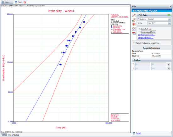
- [math]\displaystyle{ \begin{align} & \hat{\beta }=5.76 \\ & \hat{\eta }=44.68 \\ \end{align}\,\! }[/math]
Using RRX or rank regression on X:
- [math]\displaystyle{ \begin{align} & \hat{\beta }=5.70 \\ & \hat{\eta }=44.54 \\ \end{align}\,\! }[/math]
Using RRY or rank regression on Y:
- [math]\displaystyle{ \begin{align} & \hat{\beta }=5.41 \\ & \hat{\eta }=44.76 \\ \end{align}\,\! }[/math]
The plot of the MLE solution with the two-sided 90% confidence bounds is:
Mixed Data Types Example
From Dimitri Kececioglu, Reliability & Life Testing Handbook, Page 406. [20].
Estimate the parameters for the 3-parameter Weibull, for a sample of 10 units that are all tested to failure. The recorded failure times are 200; 370; 500; 620; 730; 840; 950; 1,050; 1,160 and 1,400 hours.
Published Results:
Published results (using probability plotting):
- [math]\displaystyle{ {\widehat{\beta}} = 3.0\,\! }[/math], [math]\displaystyle{ {\widehat{\eta}} = 1,220\,\! }[/math], [math]\displaystyle{ {\widehat{\gamma}} = -300\,\! }[/math]
Computed Results in Weibull++
Weibull++ computed parameters for rank regression on X are:
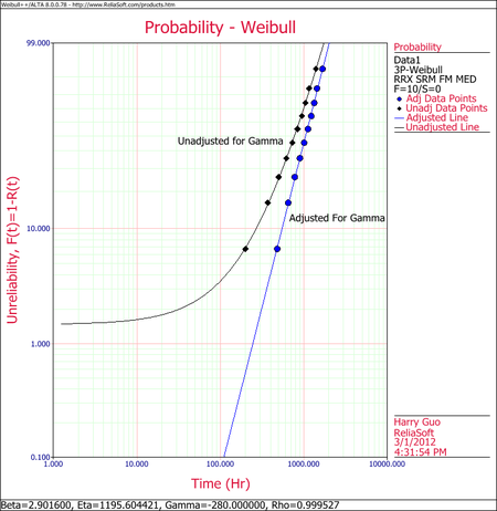
- [math]\displaystyle{ {\widehat{\beta}} = 2.9013\,\! }[/math], [math]\displaystyle{ {\widehat{\eta}} = 1195.5009\,\! }[/math], [math]\displaystyle{ {\widehat{\gamma}} = -279.000\,\! }[/math]
The small difference between the published results and the ones obtained from Weibull++ are due to the difference in the estimation method. In the publication the parameters were estimated using probability plotting (i.e., the fitted line was "eye-balled"). In Weibull++, the parameters were estimated using non-linear regression (a more accurate, mathematically fitted line). Note that γ in this example is negative. This means that the unadjusted for γ line is concave up, as shown next.
Weibull Distribution RRX Example
Assume that 6 identical units are being tested. The failure times are: 93, 34, 16, 120, 53 and 75 hours.
1. What is the unreliability of the units for a mission duration of 30 hours, starting the mission at age zero?
2. What is the reliability for a mission duration of 10 hours, starting the new mission at the age of T = 30 hours?
3. What is the longest mission that this product should undertake for a reliability of 90%?
Solution
1. First, we use Weibull++ to obtain the parameters using RRX.
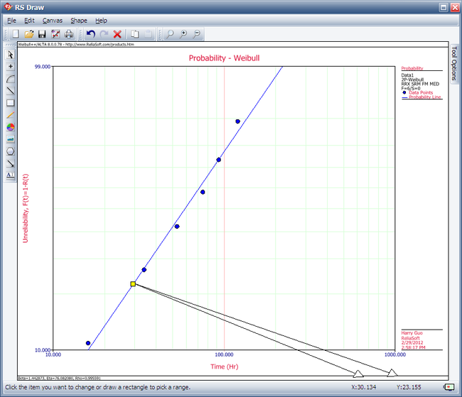
Then, we investigate several methods of solution for this problem. The first, and more laborious, method is to extract the information directly from the plot. You may do this with either the screen plot in RS Draw or the printed copy of the plot. (When extracting information from the screen plot in RS Draw, note that the translated axis position of your mouse is always shown on the bottom right corner.)
Using this first method, enter either the screen plot or the printed plot with T = 30 hours, go up vertically to the straight line fitted to the data, then go horizontally to the ordinate, and read off the result. A good estimate of the unreliability is 23%. (Also, the reliability estimate is 1.0 - 0.23 = 0.77 or 77%.)
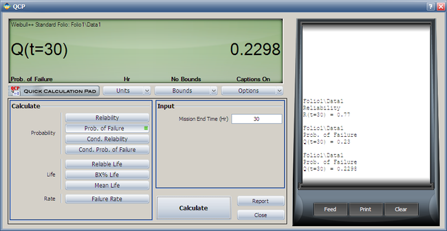
The second method involves the use of the Quick Calculation Pad (QCP).
Select the Prob. of Failure calculation option and enter 30 hours in the Mission End Time field.
Note that the results in QCP vary according to the parameter estimation method used. The above results are obtained using RRX.
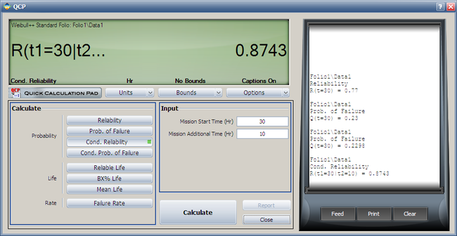
2. The conditional reliability is given by:
- [math]\displaystyle{ R(t|T)=\frac{R(T+t)}{R(T)}\,\! }[/math]
or:
- [math]\displaystyle{ \hat{R}(10hr|30hr)=\frac{\hat{R}(10+30)}{\hat{R}(30)}=\frac{\hat{R}(40)}{\hat{R}(30)}\,\! }[/math]
Again, the QCP can provide this result directly and more accurately than the plot.
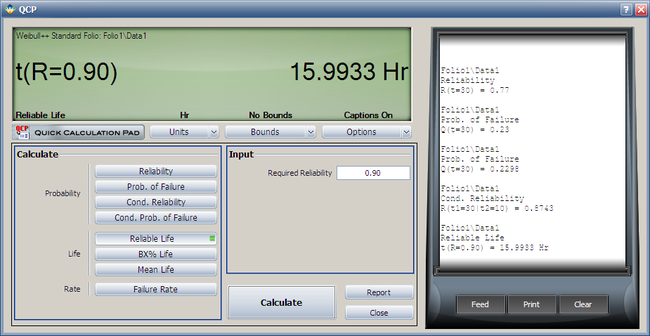
3. To use the QCP to solve for the longest mission that this product should undertake for a reliability of 90%, choose Reliable Life and enter 0.9 for the required reliability. The result is 15.9933 hours.
Benchmark with Published Examples
The following examples compare published results to computed results obtained with Weibull++.
Complete Data RRY Example
From Dimitri Kececioglu, Reliability & Life Testing Handbook, Page 418 [20].
Sample of 10 units, all tested to failure. The failures were recorded at 16, 34, 53, 75, 93, 120, 150, 191, 240 and 339 hours.
Published Results
Published Results (using Rank Regression on Y):
- [math]\displaystyle{ \begin{align} & \widehat{\beta }=1.20 \\ & \widehat{\eta} = 146.2 \\ & \hat{\rho }=0.998703\\ \end{align}\,\! }[/math]
Computed Results in Weibull++
This same data set can be entered into a Weibull++ standard data sheet. Use RRY for the estimation method.
Weibull++ computed parameters for RRY are:
- [math]\displaystyle{ \begin{align} & \widehat{\beta }=1.1973 \\ & \widehat{\eta} = 146.2545 \\ & \hat{\rho }=0.9999\\ \end{align}\,\! }[/math]
The small difference between the published results and the ones obtained from Weibull++ is due to the difference in the median rank values between the two (in the publication, median ranks are obtained from tables to 3 decimal places, whereas in Weibull++ they are calculated and carried out up to the 15th decimal point).
You will also notice that in the examples that follow, a small difference may exist between the published results and the ones obtained from Weibull++. This can be attributed to the difference between the computer numerical precision employed by Weibull++ and the lower number of significant digits used by the original authors. In most of these publications, no information was given as to the numerical precision used.
Suspension Data MLE Example
From Wayne Nelson, Fan Example, Applied Life Data Analysis, page 317 [30].
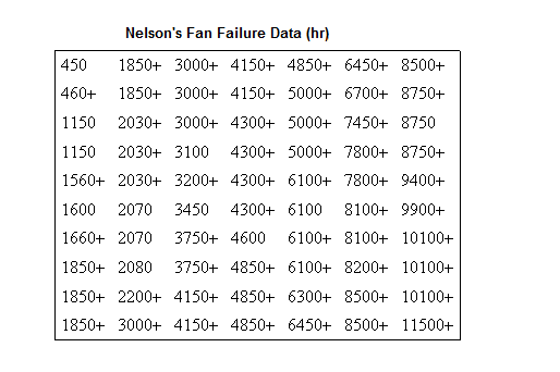
70 diesel engine fans accumulated 344,440 hours in service and 12 of them failed. A table of their life data is shown next (+ denotes non-failed units or suspensions, using Dr. Nelson's nomenclature). Evaluate the parameters with their two-sided 95% confidence bounds, using MLE for the 2-parameter Weibull distribution.
Published Results:
Weibull parameters (2P-Weibull, MLE):
- [math]\displaystyle{ \begin{align} & \widehat{\beta }=1.0584 \\ & \widehat{\eta} = 26,296 \\ \end{align}\,\! }[/math]
Published 95% FM confidence limits on the parameters:
- [math]\displaystyle{ \begin{align} & \widehat{\beta }=\lbrace 0.6441, \text{ }1.7394\rbrace \\ & \widehat{\eta} = \lbrace 10,522, \text{ }65,532\rbrace \\ \end{align}\,\! }[/math]
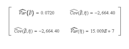
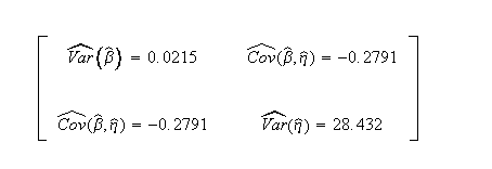
Published variance/covariance matrix:
Note that Nelson expresses the results as multiples of 1,000 (or = 26.297, etc.). The published results were adjusted by this factor to correlate with Weibull++ results.
Computed Results in Weibull++
This same data set can be entered into a Weibull++ standard folio, using 2-parameter Weibull and MLE to calculate the parameter estimates.
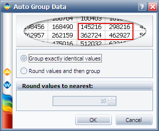
You can also enter the data as given in table without grouping them by opening a data sheet configured for suspension data. Then click the Group Data icon and chose Group exactly identical values.
The data will be automatically grouped and put into a new grouped data sheet.
Weibull++ computed parameters for maximum likelihood are:
- [math]\displaystyle{ \begin{align} & \widehat{\beta }=1.0584 \\ & \widehat{\eta} = 26,297 \\ \end{align}\,\! }[/math]
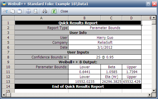
Weibull++ computed 95% FM confidence limits on the parameters:
- [math]\displaystyle{ \begin{align} & \widehat{\beta }=\lbrace 0.6441, \text{ }1.7394\rbrace \\ & \widehat{\eta} = \lbrace 10,522, \text{ }65,532\rbrace \\ \end{align}\,\! }[/math]
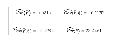
Weibull++ computed/variance covariance matrix:
The two-sided 95% bounds on the parameters can be determined from the QCP. Calculate and then click Report to see the results.
Interval Data MLE Example
From Wayne Nelson, Applied Life Data Analysis, Page 415 [30]. 167 identical parts were inspected for cracks. The following is a table of their last inspection times and times-to-failure:
Published Results:
Published results (using MLE):
- [math]\displaystyle{ \begin{align} & \widehat{\beta }=1.486 \\ & \widehat{\eta} = 71.687\\ \end{align}\,\! }[/math]
Published 95% FM confidence limits on the parameters:
- [math]\displaystyle{ \begin{align} & \widehat{\beta }=\lbrace 1.224, \text{ }1.802\rbrace \\ & \widehat{\eta} = \lbrace 61.962, \text{ }82.938\rbrace \\ \end{align}\,\! }[/math]
Published variance/covariance matrix:
Computed Results in Weibull++
This same data set can be entered into a Weibull++ standard folio that's configured for grouped times-to-failure data with suspensions and interval data.
Weibull++ computed parameters for maximum likelihood are:
- [math]\displaystyle{ \begin{align} & \widehat{\beta }=1.485 \\ & \widehat{\eta} = 71.690\\ \end{align}\,\! }[/math]
Weibull++ computed 95% FM confidence limits on the parameters:
- [math]\displaystyle{ \begin{align} & \widehat{\beta }=\lbrace 1.224, \text{ }1.802\rbrace \\ & \widehat{\eta} = \lbrace 61.961, \text{ }82.947\rbrace \\ \end{align}\,\! }[/math]
Weibull++ computed/variance covariance matrix:
Grouped Suspension MLE Example
From Dallas R. Wingo, IEEE Transactions on Reliability Vol. R-22, No 2, June 1973, Pages 96-100.
Wingo uses the following times-to-failure: 37, 55, 64, 72, 74, 87, 88, 89, 91, 92, 94, 95, 97, 98, 100, 101, 102, 102, 105, 105, 107, 113, 117, 120, 120, 120, 122, 124, 126, 130, 135, 138, 182. In addition, the following suspensions are used: 4 at 70, 5 at 80, 4 at 99, 3 at 121 and 1 at 150.
Published Results (using MLE)
- [math]\displaystyle{ \begin{align} & \widehat{\beta }=3.7596935\\ & \widehat{\eta} = 106.49758 \\ & \hat{\gamma }=14.451684\\ \end{align}\,\! }[/math]
Computed Results in Weibull++
- [math]\displaystyle{ \begin{align} & \widehat{\beta }=3.7596935\\ & \widehat{\eta} = 106.49758 \\ & \hat{\gamma }=14.451684\\ \end{align}\,\! }[/math]
Note that you must select the Use True 3-P MLEoption in the Weibull++ Application Setup to replicate these results.
3-P Probability Plot Example
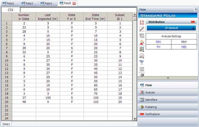
Suppose we want to model a left censored, right censored, interval, and complete data set, consisting of 274 units under test of which 185 units fail. The following table contains the data.
| Data Point Index | Number in State | Last Inspection | State (S or F) | State End Time |
| 1 | 2 | 5 | F | 5 |
| 2 | 23 | 5 | S | 5 |
| 3 | 28 | 0 | F | 7 |
| 4 | 4 | 10 | F | 10 |
| 5 | 7 | 15 | F | 15 |
| 6 | 8 | 20 | F | 20 |
| 7 | 29 | 20 | S | 20 |
| 8 | 32 | 0 | F | 22 |
| 9 | 6 | 25 | F | 25 |
| 10 | 4 | 27 | F | 30 |
| 11 | 8 | 30 | F | 35 |
| 12 | 5 | 30 | F | 40 |
| 13 | 9 | 27 | F | 45 |
| 14 | 7 | 25 | F | 50 |
| 15 | 5 | 20 | F | 55 |
| 16 | 3 | 15 | F | 60 |
| 17 | 6 | 10 | F | 65 |
| 18 | 3 | 5 | F | 70 |
| 19 | 37 | 100 | S | 100 |
| 20 | 48 | 0 | F | 102 |
Solution
Since standard ranking methods for dealing with these different data types are inadequate, we will want to use the ReliaSoft ranking method. This option is the default in Weibull++ when dealing with interval data. The filled-out standard folio is shown next:
The computed parameters using MLE are:
- [math]\displaystyle{ \hat{\beta }=0.748;\text{ }\hat{\eta }=44.38\,\! }[/math]
Using RRX:
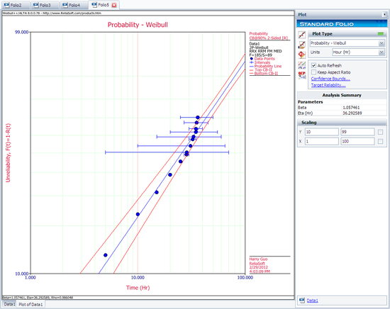
- [math]\displaystyle{ \hat{\beta }=1.057;\text{ }\hat{\eta }=36.29\,\! }[/math]
Using RRY:
- [math]\displaystyle{ \hat{\beta }=0.998;\text{ }\hat{\eta }=37.16\,\! }[/math]
The plot with the two-sided 90% confidence bounds for the rank regression on X solution is:

