Normal Distribution Examples: Difference between revisions
Kate Racaza (talk | contribs) No edit summary |
Lisa Hacker (talk | contribs) No edit summary |
||
| (25 intermediate revisions by 4 users not shown) | |||
| Line 1: | Line 1: | ||
<noinclude>{{Banner Weibull Examples}}{{Navigation box}} | <noinclude>{{Banner Weibull Examples}}{{Navigation box}} | ||
''These examples appear in the [[ | ''These examples appear in the [https://help.reliasoft.com/reference/life_data_analysis Life data analysis reference].'' | ||
</noinclude> | |||
The following examples illustrate the different types of life data that can be analyzed in Weibull++ using the normal distribution. For more information on the different types of life data, see [[Life Data Classification]]. | |||
===Complete Data Example=== | |||
The following | 6 units are tested to failure. The following failure times data are obtained: 12125, 11260, 12080, 12825, 13550 and 14670 hours. Assuming that the data are normally distributed, do the following: | ||
'''Objectives''' | |||
:1. Find the parameters for the data set, using the Rank Regression on X (RRX) parameter estimation method | :1. Find the parameters for the data set, using the Rank Regression on X (RRX) parameter estimation method | ||
:2. Obtain the probability plot for the data with 90%, two-sided Type 1 confidence bounds. | :2. Obtain the probability plot for the data with 90%, two-sided Type 1 confidence bounds. | ||
:3. Obtain the | :3. Obtain the ''pdf'' plot for the data. | ||
:4. Using the Quick Calculation Pad, determine the reliability for a mission of 11,000 hours, as well as the upper and lower two-sided 90% confidence limit on this reliability. | :4. Using the Quick Calculation Pad (QCP), determine the reliability for a mission of 11,000 hours, as well as the upper and lower two-sided 90% confidence limit on this reliability. | ||
:5 | :5. Using the QCP, determine the MTTF, as well as the upper and lower two-sided 90% confidence limit on this MTTF. | ||
:6. Obtain tabulated values for the failure rate for 10 different mission end times. The mission end times are 1,000 to 10,000 hours, using increments of 1,000 hours. | |||
| Line 22: | Line 24: | ||
[[Image:Normal Distribution Example 8 Data.png|center| | [[Image:Normal Distribution Example 8 Data.png|center|650px| ]] | ||
The following figures show the probability plot with the 90% two-sided confidence bounds and the | The following figures show the probability plot with the 90% two-sided confidence bounds and the ''pdf'' plot. | ||
| Line 37: | Line 39: | ||
[[Image:Normal Distribution Example 9 QCP 1.png|center|550px| ]] | [[Image:Normal Distribution Example 9 QCP 1.png|center|650px| ]] | ||
[[Image:Normal Distribution Example 9 QCP 2.png|center|650px| ]] | |||
To obtain tabulated values for the failure rate, use the Analysis Workbook or General Spreadsheet features that are included in Weibull++. (For more information on these features, please refer to the Weibull++ User's Guide. For a step-by-step example on creating Weibull++ reports, please see the [http://www.reliasoft.tv/weibull/startguide/weibull_qsg_2.html Quick Start Guide]). The following worksheet shows the mission times and the corresponding failure rates. | |||
[[Image:folio^E.png|center|550px]] | |||
===Suspension Data Example=== | |||
19 units are being reliability tested and the following is a table of their times-to-failure and suspensions. | |||
{|border="1" align="center" style="border-collapse: collapse;" cellpadding="5" cellspacing="5" | |||
|- | |||
|colspan="3" style="text-align:center"| '''Non-Grouped Data Times-to-Failure Data with Suspensions''' | |||
|- | |||
!Data point index | |||
!Last Inspected | |||
!State End Time | |||
|- | |||
|1 ||F||2 | |||
|- | |||
|2 ||S||3 | |||
|- | |||
|3 ||F||5 | |||
|- | |||
|4 ||S||7 | |||
|- | |||
|5 ||F||11 | |||
|- | |||
|6 ||S||13 | |||
|- | |||
|7||S||17 | |||
|- | |||
|8||S||19 | |||
|- | |||
|9 ||F||23 | |||
|- | |||
|10 ||F||29 | |||
|- | |||
|11 ||S||31 | |||
|- | |||
|12 ||F||37 | |||
|- | |||
|13 ||S||41 | |||
|- | |||
|14 ||F||43 | |||
|- | |||
|15||S||47 | |||
|- | |||
|16||S||53 | |||
|- | |||
|17||F||59 | |||
|- | |||
|18||S||61 | |||
|- | |||
|19||S||67 | |||
|} | |||
Using the normal distribution and the maximum likelihood (MLE) parameter estimation method, the computed parameters are: | |||
::<math>\begin{align} | |||
& \widehat{\mu }= & 48.07 \\ | |||
& {{{\hat{\sigma }}}_{T}}= & 28.41. | |||
\end{align}\,\!</math> | |||
If we analyze the data set with the rank regression on x (RRX) method, the computed parameters are: | |||
::<math>\begin{align} | |||
& \widehat{\mu }= & 46.40 \\ | |||
& {{{\hat{\sigma }}}_{T}}= & 28.64. | |||
\end{align}\,\!</math> | |||
For the rank regression on y (RRY) method, the parameters are: | |||
::<math>\begin{align} | |||
& \widehat{\mu }= & 47.34 \\ | |||
& {{{\hat{\sigma }}}_{T}}= & 29.96. | |||
\end{align}\,\!</math> | |||
===Interval Censored Data Example=== | |||
8 units are being reliability tested, and the following is a table of their failure times: | |||
{|border="1" align="center" style="border-collapse: collapse;" cellpadding="5" cellspacing="5" | |||
|- | |||
|colspan="3" style="text-align:center"| '''Non-Grouped Interval Data''' | |||
|- | |||
!Data point index | |||
!Last Inspected | |||
!State End Time | |||
|- | |||
|1 ||30||32 | |||
|- | |||
|2 ||32||35 | |||
|- | |||
|3 ||35||37 | |||
|- | |||
|4 ||37||40 | |||
|- | |||
|5 ||42||42 | |||
|- | |||
|6 ||45||45 | |||
|- | |||
|7||50||50 | |||
|- | |||
|8||55||55 | |||
|} | |||
This is a sequence of interval times-to-failure data. Using the normal distribution and the maximum likelihood (MLE) parameter estimation method, the computed parameters are: | |||
::<math>\begin{align} | |||
& \widehat{\mu }= & 41.40 \\ | |||
& {{{\hat{\sigma }}}_{T}}= & 7.740. | |||
\end{align}\,\!</math> | |||
For rank regression on x: | |||
::<math>\begin{align} | |||
& \widehat{\mu }= & 41.40 \\ | |||
& {{{\hat{\sigma }}}_{T}}= & 9.03. | |||
\end{align}\,\!</math> | |||
If we analyze the data set with the rank regression on y (RRY) parameter estimation method, the computed parameters are: | |||
::<math>\begin{align} | |||
& \widehat{\mu }= & 41.39 \\ | |||
& {{{\hat{\sigma }}}_{T}}= & 9.25. | |||
\end{align}\,\!</math> | |||
The following plot shows the results if the data were analyzed using the rank regression on X (RRX) method. | |||
[[Image:lastinspectedplot.png|center|600px| ]] | |||
===Mixed Data Types Example=== | |||
Suppose our data set includes left and right censored, interval censored and complete data, as shown in the following table. | |||
{|border="1" align="center" style="border-collapse: collapse;" cellpadding="5" cellspacing="5" | |||
|- | |||
!colspan="5" style="text-align:center"| Grouped Data Times-to-Failure with Suspensions and Intervals (Interval, Left and Right Censored) | |||
|- | |||
!Data point index | |||
!Number in State | |||
!Last Inspection | |||
!State (S or F) | |||
!State End Time | |||
|- | |||
|1 ||1 ||10 ||F||10 | |||
|- | |||
|2 ||1 ||20 ||S||20 | |||
|- | |||
|3 ||2 ||0 ||F||30 | |||
|- | |||
|4 ||2 ||40 ||F||40 | |||
|- | |||
|5 ||1 ||50 ||F||50 | |||
|- | |||
|6 ||1 ||60 ||S||60 | |||
|- | |||
|7 ||1 ||70 ||F||70 | |||
|- | |||
|8 ||2 ||20 ||F||80 | |||
|- | |||
|9 ||1 ||10 ||F||85 | |||
|- | |||
|10||1 ||100||F||100 | |||
|} | |||
Using the normal distribution and the maximum likelihood (MLE) parameter estimation method, the computed parameters are: | |||
::<math>\begin{align} | |||
& \widehat{\mu }= & 48.11 \\ | |||
& {{{\hat{\sigma }}}_{T}}= & 26.42 | |||
\end{align}\,\!</math> | |||
If we analyze the data set with the rank regression on x (RRX) method, the computed parameters are: | |||
== | ::<math>\begin{align} | ||
& \widehat{\mu }= & 49.99 \\ | |||
& {{{\hat{\sigma }}}_{T}}= & 30.17 | |||
\end{align}\,\!</math> | |||
For the rank regression on y (RRY) method, the parameters are: | |||
=== | ::<math>\begin{align} | ||
& \widehat{\mu }= & 51.61 \\ | |||
& {{{\hat{\sigma }}}_{T}}= & 33.07 | |||
\end{align}\,\!</math> | |||
===Comparison of Analysis Methods=== | |||
8 units are being reliability tested, and the following is a table of their failure times: | |||
{|border="1" align="center" style="border-collapse: collapse;" cellpadding="5" cellspacing="5" | |||
|- | |||
|colspan="3" style="text-align:center"| '''Non-Grouped Times-to-Failure Data''' | |||
|- | |||
!Data point index | |||
!State F or S | |||
!State End Time | |||
|- | |||
|1 ||F||2 | |||
|- | |||
|2 ||F||5 | |||
|- | |||
|3 ||F||11 | |||
|- | |||
|4 ||F||23 | |||
|- | |||
|5 ||F||29 | |||
|- | |||
|6 ||F||37 | |||
|- | |||
|7||F||43 | |||
|- | |||
|8||F||59 | |||
|} | |||
Using the normal distribution and the maximum likelihood (MLE) parameter estimation method, the computed parameters are: | |||
< | ::<math>\begin{align} | ||
{{ | & \widehat{\mu }= & 26.13 \\ | ||
& {{{\hat{\sigma }}}_{T}}= & 18.57 | |||
\end{align}\,\!</math> | |||
If we analyze the data set with the rank regression on x (RRX) method, the computed parameters are: | |||
< | ::<math>\begin{align} | ||
{{ | & \widehat{\mu }= & 26.13 \\ | ||
& {{{\hat{\sigma }}}_{T}}= & 21.64 | |||
\end{align}\,\!</math> | |||
For the rank regression on y (RRY) method, the parameters are: | |||
< | ::<math>\begin{align} | ||
{{ | & \widehat{\mu }= & 26.13 \\ | ||
& {{{\hat{\sigma }}}_{T}}= & 22.28. | |||
\end{align}\,\!</math> | |||
Latest revision as of 21:45, 18 September 2023
New format available! This reference is now available in a new format that offers faster page load, improved display for calculations and images and more targeted search.
As of January 2024, this Reliawiki page will not continue to be updated. Please update all links and bookmarks to the latest references at Weibull examples and Weibull reference examples.
These examples appear in the Life data analysis reference.
The following examples illustrate the different types of life data that can be analyzed in Weibull++ using the normal distribution. For more information on the different types of life data, see Life Data Classification.
Complete Data Example
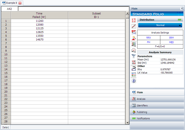
6 units are tested to failure. The following failure times data are obtained: 12125, 11260, 12080, 12825, 13550 and 14670 hours. Assuming that the data are normally distributed, do the following:
Objectives
- 1. Find the parameters for the data set, using the Rank Regression on X (RRX) parameter estimation method
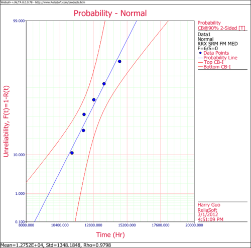
- 2. Obtain the probability plot for the data with 90%, two-sided Type 1 confidence bounds.
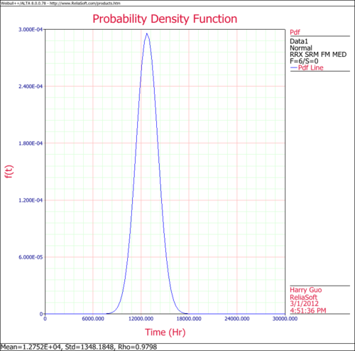
- 3. Obtain the pdf plot for the data.
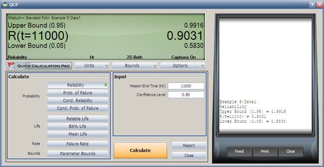
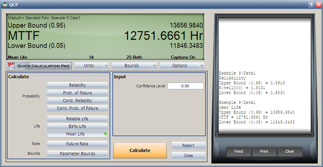
- 4. Using the Quick Calculation Pad (QCP), determine the reliability for a mission of 11,000 hours, as well as the upper and lower two-sided 90% confidence limit on this reliability.
- 5. Using the QCP, determine the MTTF, as well as the upper and lower two-sided 90% confidence limit on this MTTF.
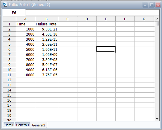
- 6. Obtain tabulated values for the failure rate for 10 different mission end times. The mission end times are 1,000 to 10,000 hours, using increments of 1,000 hours.
Solution
The following figure shows the data as entered in Weibull++, as well as the calculated parameters.
The following figures show the probability plot with the 90% two-sided confidence bounds and the pdf plot.
Both the reliability and MTTF can be easily obtained from the QCP. The QCP, with results, for both cases is shown in the next two figures.
To obtain tabulated values for the failure rate, use the Analysis Workbook or General Spreadsheet features that are included in Weibull++. (For more information on these features, please refer to the Weibull++ User's Guide. For a step-by-step example on creating Weibull++ reports, please see the Quick Start Guide). The following worksheet shows the mission times and the corresponding failure rates.
Suspension Data Example
19 units are being reliability tested and the following is a table of their times-to-failure and suspensions.
| Non-Grouped Data Times-to-Failure Data with Suspensions | ||
| Data point index | Last Inspected | State End Time |
|---|---|---|
| 1 | F | 2 |
| 2 | S | 3 |
| 3 | F | 5 |
| 4 | S | 7 |
| 5 | F | 11 |
| 6 | S | 13 |
| 7 | S | 17 |
| 8 | S | 19 |
| 9 | F | 23 |
| 10 | F | 29 |
| 11 | S | 31 |
| 12 | F | 37 |
| 13 | S | 41 |
| 14 | F | 43 |
| 15 | S | 47 |
| 16 | S | 53 |
| 17 | F | 59 |
| 18 | S | 61 |
| 19 | S | 67 |
Using the normal distribution and the maximum likelihood (MLE) parameter estimation method, the computed parameters are:
- [math]\displaystyle{ \begin{align} & \widehat{\mu }= & 48.07 \\ & {{{\hat{\sigma }}}_{T}}= & 28.41. \end{align}\,\! }[/math]
If we analyze the data set with the rank regression on x (RRX) method, the computed parameters are:
- [math]\displaystyle{ \begin{align} & \widehat{\mu }= & 46.40 \\ & {{{\hat{\sigma }}}_{T}}= & 28.64. \end{align}\,\! }[/math]
For the rank regression on y (RRY) method, the parameters are:
- [math]\displaystyle{ \begin{align} & \widehat{\mu }= & 47.34 \\ & {{{\hat{\sigma }}}_{T}}= & 29.96. \end{align}\,\! }[/math]
Interval Censored Data Example
8 units are being reliability tested, and the following is a table of their failure times:
| Non-Grouped Interval Data | ||
| Data point index | Last Inspected | State End Time |
|---|---|---|
| 1 | 30 | 32 |
| 2 | 32 | 35 |
| 3 | 35 | 37 |
| 4 | 37 | 40 |
| 5 | 42 | 42 |
| 6 | 45 | 45 |
| 7 | 50 | 50 |
| 8 | 55 | 55 |
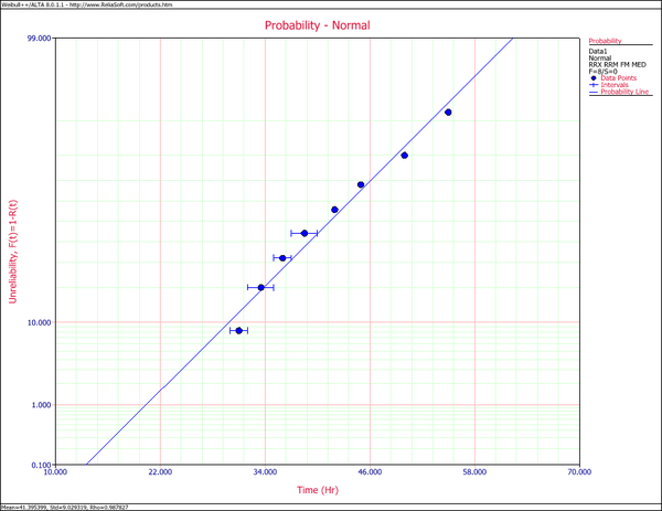
This is a sequence of interval times-to-failure data. Using the normal distribution and the maximum likelihood (MLE) parameter estimation method, the computed parameters are:
- [math]\displaystyle{ \begin{align} & \widehat{\mu }= & 41.40 \\ & {{{\hat{\sigma }}}_{T}}= & 7.740. \end{align}\,\! }[/math]
For rank regression on x:
- [math]\displaystyle{ \begin{align} & \widehat{\mu }= & 41.40 \\ & {{{\hat{\sigma }}}_{T}}= & 9.03. \end{align}\,\! }[/math]
If we analyze the data set with the rank regression on y (RRY) parameter estimation method, the computed parameters are:
- [math]\displaystyle{ \begin{align} & \widehat{\mu }= & 41.39 \\ & {{{\hat{\sigma }}}_{T}}= & 9.25. \end{align}\,\! }[/math]
The following plot shows the results if the data were analyzed using the rank regression on X (RRX) method.
Mixed Data Types Example
Suppose our data set includes left and right censored, interval censored and complete data, as shown in the following table.
| Grouped Data Times-to-Failure with Suspensions and Intervals (Interval, Left and Right Censored) | ||||
|---|---|---|---|---|
| Data point index | Number in State | Last Inspection | State (S or F) | State End Time |
| 1 | 1 | 10 | F | 10 |
| 2 | 1 | 20 | S | 20 |
| 3 | 2 | 0 | F | 30 |
| 4 | 2 | 40 | F | 40 |
| 5 | 1 | 50 | F | 50 |
| 6 | 1 | 60 | S | 60 |
| 7 | 1 | 70 | F | 70 |
| 8 | 2 | 20 | F | 80 |
| 9 | 1 | 10 | F | 85 |
| 10 | 1 | 100 | F | 100 |
Using the normal distribution and the maximum likelihood (MLE) parameter estimation method, the computed parameters are:
- [math]\displaystyle{ \begin{align} & \widehat{\mu }= & 48.11 \\ & {{{\hat{\sigma }}}_{T}}= & 26.42 \end{align}\,\! }[/math]
If we analyze the data set with the rank regression on x (RRX) method, the computed parameters are:
- [math]\displaystyle{ \begin{align} & \widehat{\mu }= & 49.99 \\ & {{{\hat{\sigma }}}_{T}}= & 30.17 \end{align}\,\! }[/math]
For the rank regression on y (RRY) method, the parameters are:
- [math]\displaystyle{ \begin{align} & \widehat{\mu }= & 51.61 \\ & {{{\hat{\sigma }}}_{T}}= & 33.07 \end{align}\,\! }[/math]
Comparison of Analysis Methods
8 units are being reliability tested, and the following is a table of their failure times:
| Non-Grouped Times-to-Failure Data | ||
| Data point index | State F or S | State End Time |
|---|---|---|
| 1 | F | 2 |
| 2 | F | 5 |
| 3 | F | 11 |
| 4 | F | 23 |
| 5 | F | 29 |
| 6 | F | 37 |
| 7 | F | 43 |
| 8 | F | 59 |
Using the normal distribution and the maximum likelihood (MLE) parameter estimation method, the computed parameters are:
- [math]\displaystyle{ \begin{align} & \widehat{\mu }= & 26.13 \\ & {{{\hat{\sigma }}}_{T}}= & 18.57 \end{align}\,\! }[/math]
If we analyze the data set with the rank regression on x (RRX) method, the computed parameters are:
- [math]\displaystyle{ \begin{align} & \widehat{\mu }= & 26.13 \\ & {{{\hat{\sigma }}}_{T}}= & 21.64 \end{align}\,\! }[/math]
For the rank regression on y (RRY) method, the parameters are:
- [math]\displaystyle{ \begin{align} & \widehat{\mu }= & 26.13 \\ & {{{\hat{\sigma }}}_{T}}= & 22.28. \end{align}\,\! }[/math]

