Crow-AMSAA Confidence Bounds Example: Difference between revisions
Chris Kahn (talk | contribs) No edit summary |
Lisa Hacker (talk | contribs) No edit summary |
||
| (10 intermediate revisions by 2 users not shown) | |||
| Line 1: | Line 1: | ||
<noinclude>{{Banner RGA Examples}} | <noinclude>{{Banner RGA Examples}} | ||
''This example appears in the [ | ''This example appears in the [https://help.reliasoft.com/reference/reliability_growth_and_repairable_system_analysis Reliability growth reference]''. | ||
</noinclude> | </noinclude> | ||
Using the values of <math>\hat{\beta }\,\!</math> and <math>\hat{\lambda }\,\!</math> estimated in the <noinclude>[[Crow-AMSAA | ====Example - Confidence Bounds on Failure Intensity==== | ||
Using the values of <math>\hat{\beta }\,\!</math> and <math>\hat{\lambda }\,\!</math> estimated in the <noinclude>[[Crow-AMSAA Parameter Estimation Example]]</noinclude><includeonly>example given above</includeonly>, calculate the 90% 2-sided confidence bounds on the cumulative and instantaneous failure intensity. | |||
'''Solution''' | '''Solution''' | ||
| Line 10: | Line 11: | ||
The partial derivatives for the Fisher Matrix confidence bounds are: | The partial derivatives for the Fisher Matrix confidence bounds are: | ||
:<math>\begin{align} | :<math>\begin{align} | ||
| Line 17: | Line 17: | ||
\frac{{{\partial }^{2}}\Lambda }{\partial \lambda \partial \beta } = & -{{620}^{0.6142}}\ln 620=-333.64 | \frac{{{\partial }^{2}}\Lambda }{\partial \lambda \partial \beta } = & -{{620}^{0.6142}}\ln 620=-333.64 | ||
\end{align}\,\!</math> | \end{align}\,\!</math> | ||
The Fisher Matrix then becomes: | The Fisher Matrix then becomes: | ||
:<math>\begin{align} | :<math>\begin{align} | ||
| Line 27: | Line 25: | ||
& = \begin{bmatrix} 0.13519969 & -0.046614609\\ -0.046614609 & 0.017105343 \end{bmatrix} | & = \begin{bmatrix} 0.13519969 & -0.046614609\\ -0.046614609 & 0.017105343 \end{bmatrix} | ||
\end{align}\,\!</math> | \end{align}\,\!</math> | ||
For <math>T=620\,\!</math> hours, the partial derivatives of the cumulative and instantaneous failure intensities are: | For <math>T=620\,\!</math> hours, the partial derivatives of the cumulative and instantaneous failure intensities are: | ||
:<math>\begin{align} | :<math>\begin{align} | ||
| Line 40: | Line 36: | ||
= & 0.083694185 | = & 0.083694185 | ||
\end{align}\,\!</math> | \end{align}\,\!</math> | ||
:<math>\begin{align} | :<math>\begin{align} | ||
| Line 47: | Line 42: | ||
= & 0.17558519 | = & 0.17558519 | ||
\end{align}\,\!</math> | \end{align}\,\!</math> | ||
:<math>\begin{align} | :<math>\begin{align} | ||
| Line 54: | Line 48: | ||
= & 0.051404969 | = & 0.051404969 | ||
\end{align}\,\!</math> | \end{align}\,\!</math> | ||
Therefore, the variances become: | Therefore, the variances become: | ||
:<math>\begin{align} | :<math>\begin{align} | ||
| Line 65: | Line 57: | ||
&= 0.0000431393 | &= 0.0000431393 | ||
\end{align}\,\!</math> | \end{align}\,\!</math> | ||
The cumulative and instantaneous failure intensities at <math>T=620\,\!</math> hours are: | The cumulative and instantaneous failure intensities at <math>T=620\,\!</math> hours are: | ||
:<math>\begin{align} | :<math>\begin{align} | ||
| Line 74: | Line 64: | ||
{{\lambda }_{i}}(T)= & 0.02179 | {{\lambda }_{i}}(T)= & 0.02179 | ||
\end{align}\,\!</math> | \end{align}\,\!</math> | ||
So, at the 90% confidence level and for <math>T=620\,\!</math> hours, the Fisher Matrix confidence bounds for the cumulative failure intensity are: | So, at the 90% confidence level and for <math>T=620\,\!</math> hours, the Fisher Matrix confidence bounds for the cumulative failure intensity are: | ||
:<math>\begin{align} | :<math>\begin{align} | ||
| Line 83: | Line 71: | ||
{{[{{\lambda }_{c}}(T)]}_{U}}= & 0.05039 | {{[{{\lambda }_{c}}(T)]}_{U}}= & 0.05039 | ||
\end{align}\,\!</math> | \end{align}\,\!</math> | ||
The confidence bounds for the instantaneous failure intensity are: | The confidence bounds for the instantaneous failure intensity are: | ||
:<math>\begin{align} | :<math>\begin{align} | ||
| Line 92: | Line 78: | ||
{{[{{\lambda }_{i}}(T)]}_{U}}= & 0.03579 | {{[{{\lambda }_{i}}(T)]}_{U}}= & 0.03579 | ||
\end{align}\,\!</math> | \end{align}\,\!</math> | ||
The following figures display plots of the Fisher Matrix confidence bounds for the cumulative and instantaneous failure intensity, respectively. | The following figures display plots of the Fisher Matrix confidence bounds for the cumulative and instantaneous failure intensity, respectively. | ||
[[Image:rga5.2.png|center|450px]] | |||
[[Image:rga5.3.png|center|450px]] | |||
[[Image:rga5.3.png|center| | |||
'''Crow Bounds''' | '''Crow Bounds''' | ||
Given that the data is failure terminated, the Crow confidence bounds for the cumulative failure intensity at the 90% confidence level and for <math>T=620\,\!</math> hours are: | Given that the data is failure terminated, the Crow confidence bounds for the cumulative failure intensity at the 90% confidence level and for <math>T=620\,\!</math> hours are: | ||
:<math>\begin{align} | :<math>\begin{align} | ||
| Line 116: | Line 97: | ||
= & 0.048775 | = & 0.048775 | ||
\end{align}\,\!</math> | \end{align}\,\!</math> | ||
The Crow confidence bounds for the instantaneous failure intensity at the 90% confidence level and for <math>T=620\,\!</math> hours are calculated by first estimating the bounds on the instantaneous MTBF. Once these are calculated, take the inverse as shown below. Details on the confidence bounds for instantaneous MTBF are presented [[Crow-AMSAA Confidence Bounds#Crow_Bounds_4|here]]. | The Crow confidence bounds for the instantaneous failure intensity at the 90% confidence level and for <math>T=620\,\!</math> hours are calculated by first estimating the bounds on the instantaneous MTBF. Once these are calculated, take the inverse as shown below. Details on the confidence bounds for instantaneous MTBF are presented [[Crow-AMSAA Confidence Bounds#Crow_Bounds_4|here]]. | ||
:<math>\begin{align} | :<math>\begin{align} | ||
| Line 126: | Line 105: | ||
= & 0.01179 | = & 0.01179 | ||
\end{align}\,\!</math> | \end{align}\,\!</math> | ||
:<math>\begin{align} | :<math>\begin{align} | ||
| Line 133: | Line 111: | ||
= & 0.03253 | = & 0.03253 | ||
\end{align}\,\!</math> | \end{align}\,\!</math> | ||
The following figures display plots of the Crow confidence bounds for the cumulative and instantaneous failure intensity, respectively. | The following figures display plots of the Crow confidence bounds for the cumulative and instantaneous failure intensity, respectively. | ||
[[Image:rga5.4.png|center|450px]] | |||
[[Image:rga5. | [[Image:rga5.5.png|center|450px]] | ||
====Example - Confidence Bounds on MTBF==== | |||
==== | |||
Calculate the confidence bounds on the cumulative and instantaneous MTBF for the data from the example given above. | Calculate the confidence bounds on the cumulative and instantaneous MTBF for the data from the example given above. | ||
| Line 152: | Line 126: | ||
From the previous example: | From the previous example: | ||
:<math>\begin{align} | :<math>\begin{align} | ||
| Line 159: | Line 132: | ||
Cov(\hat{\beta },\hat{\lambda }) = & -0.046614609 | Cov(\hat{\beta },\hat{\lambda }) = & -0.046614609 | ||
\end{align}\,\!</math> | \end{align}\,\!</math> | ||
And for <math>T=620\,\!</math> hours, the partial derivatives of the cumulative and instantaneous MTBF are: | And for <math>T=620\,\!</math> hours, the partial derivatives of the cumulative and instantaneous MTBF are: | ||
:<math>\begin{align} | :<math>\begin{align} | ||
| Line 178: | Line 149: | ||
= & -108.26001 | = & -108.26001 | ||
\end{align}\,\!</math> | \end{align}\,\!</math> | ||
Therefore, the variances become: | Therefore, the variances become: | ||
:<math>\begin{align} | :<math>\begin{align} | ||
| Line 188: | Line 157: | ||
= & 36.113376 | = & 36.113376 | ||
\end{align}\,\!</math> | \end{align}\,\!</math> | ||
:<math>\begin{align} | :<math>\begin{align} | ||
| Line 195: | Line 163: | ||
= & 191.33709 | = & 191.33709 | ||
\end{align}\,\!</math> | \end{align}\,\!</math> | ||
So, at 90% confidence level and <math>T=620\,\!</math> hours, the Fisher Matrix confidence bounds are: | So, at 90% confidence level and <math>T=620\,\!</math> hours, the Fisher Matrix confidence bounds are: | ||
:<math>\begin{align} | :<math>\begin{align} | ||
| Line 206: | Line 172: | ||
= & 40.01927 | = & 40.01927 | ||
\end{align}\,\!</math> | \end{align}\,\!</math> | ||
:<math>\begin{align} | :<math>\begin{align} | ||
| Line 214: | Line 179: | ||
= & 75.34193 | = & 75.34193 | ||
\end{align}\,\!</math> | \end{align}\,\!</math> | ||
The following two figures show plots of the Fisher Matrix confidence bounds for the cumulative and instantaneous MTBFs. | The following two figures show plots of the Fisher Matrix confidence bounds for the cumulative and instantaneous MTBFs. | ||
[[Image:rga5.6.png|center|450px]] | |||
[[Image:rga5.7.png|center|450px]] | |||
[[Image:rga5.7.png|center| | |||
'''Crow Bounds''' | '''Crow Bounds''' | ||
The Crow confidence bounds for the cumulative MTBF and the instantaneous MTBF at the 90% confidence level and for <math>T=620\,\!</math> hours are: | The Crow confidence bounds for the cumulative MTBF and the instantaneous MTBF at the 90% confidence level and for <math>T=620\,\!</math> hours are: | ||
:<math>\begin{align} | :<math>\begin{align} | ||
| Line 236: | Line 196: | ||
= & 41.6282 | = & 41.6282 | ||
\end{align}\,\!</math> | \end{align}\,\!</math> | ||
:<math>\begin{align} | :<math>\begin{align} | ||
| Line 244: | Line 203: | ||
= & 84.7972 | = & 84.7972 | ||
\end{align}\,\!</math> | \end{align}\,\!</math> | ||
The figures below show plots of the Crow confidence bounds for the cumulative and instantaneous MTBF. | The figures below show plots of the Crow confidence bounds for the cumulative and instantaneous MTBF. | ||
[[Image:rga5.8.png|center| | [[Image:rga5.8.png|center|450px]] | ||
[[Image:rga5.9.png|center|450px]] | |||
[[Image:rga5.9.png|center| | |||
Confidence bounds can also be obtained on the parameters <math>\hat{\beta }\,\!</math> and <math>\hat{\lambda }\,\!</math>. For Fisher Matrix confidence bounds: | Confidence bounds can also be obtained on the parameters <math>\hat{\beta }\,\!</math> and <math>\hat{\lambda }\,\!</math>. For Fisher Matrix confidence bounds: | ||
:<math>\begin{align} | :<math>\begin{align} | ||
| Line 262: | Line 218: | ||
= & 0.8722 | = & 0.8722 | ||
\end{align}\,\!</math> | \end{align}\,\!</math> | ||
and: | and: | ||
:<math>\begin{align} | :<math>\begin{align} | ||
| Line 273: | Line 227: | ||
= & 1.7691 | = & 1.7691 | ||
\end{align}\,\!</math> | \end{align}\,\!</math> | ||
For Crow confidence bounds: | For Crow confidence bounds: | ||
:<math>\begin{align} | :<math>\begin{align} | ||
| Line 282: | Line 234: | ||
{{\beta }_{U}}= & 0.9350 | {{\beta }_{U}}= & 0.9350 | ||
\end{align}\,\!</math> | \end{align}\,\!</math> | ||
and: | and: | ||
:<math>\begin{align} | :<math>\begin{align} | ||
Latest revision as of 21:31, 18 September 2023
New format available! This reference is now available in a new format that offers faster page load, improved display for calculations and images and more targeted search.
As of January 2024, this Reliawiki page will not continue to be updated. Please update all links and bookmarks to the latest references at RGA examples and RGA reference examples.
This example appears in the Reliability growth reference.
Example - Confidence Bounds on Failure Intensity
Using the values of [math]\displaystyle{ \hat{\beta }\,\! }[/math] and [math]\displaystyle{ \hat{\lambda }\,\! }[/math] estimated in the Crow-AMSAA Parameter Estimation Example, calculate the 90% 2-sided confidence bounds on the cumulative and instantaneous failure intensity.
Solution
Fisher Matrix Bounds
The partial derivatives for the Fisher Matrix confidence bounds are:
- [math]\displaystyle{ \begin{align} \frac{{{\partial }^{2}}\Lambda }{\partial {{\lambda }^{2}}} = & -\frac{22}{{{0.4239}^{2}}}=-122.43 \\ \frac{{{\partial }^{2}}\Lambda }{\partial {{\beta }^{2}}} = & -\frac{22}{{{0.6142}^{2}}}-0.4239\cdot {{620}^{0.6142}}{{(\ln 620)}^{2}}=-967.68 \\ \frac{{{\partial }^{2}}\Lambda }{\partial \lambda \partial \beta } = & -{{620}^{0.6142}}\ln 620=-333.64 \end{align}\,\! }[/math]
The Fisher Matrix then becomes:
- [math]\displaystyle{ \begin{align} \begin{bmatrix}122.43 & 333.64\\ 333.64 & 967.68\end{bmatrix}^{-1} & = \begin{bmatrix}Var(\hat{\lambda}) & Cov(\hat{\beta},\hat{\lambda})\\ Cov(\hat{\beta},\hat{\lambda}) & Var(\hat{\beta})\end{bmatrix} \\ & = \begin{bmatrix} 0.13519969 & -0.046614609\\ -0.046614609 & 0.017105343 \end{bmatrix} \end{align}\,\! }[/math]
For [math]\displaystyle{ T=620\,\! }[/math] hours, the partial derivatives of the cumulative and instantaneous failure intensities are:
- [math]\displaystyle{ \begin{align} \frac{\partial {{\lambda }_{c}}(T)}{\partial \beta }= & \hat{\lambda }{{T}^{\hat{\beta }-1}}\ln (T) \\ = & 0.4239\cdot {{620}^{-0.3858}}\ln 620 \\ = & 0.22811336 \\ \frac{\partial {{\lambda }_{c}}(T)}{\partial \lambda }= & {{T}^{\hat{\beta }-1}} \\ = & {{620}^{-0.3858}} \\ = & 0.083694185 \end{align}\,\! }[/math]
- [math]\displaystyle{ \begin{align} \frac{\partial {{\lambda }_{i}}(T)}{\partial \beta }= & \hat{\lambda }{{T}^{\hat{\beta }-1}}+\hat{\lambda }\hat{\beta }{{T}^{\hat{\beta }-1}}\ln T \\ = & 0.4239\cdot {{620}^{-0.3858}}+0.4239\cdot 0.6142\cdot {{620}^{-0.3858}}\ln 620 \\ = & 0.17558519 \end{align}\,\! }[/math]
- [math]\displaystyle{ \begin{align} \frac{\partial {{\lambda }_{i}}(T)}{\partial \lambda }= & \hat{\beta }{{T}^{\hat{\beta }-1}} \\ = & 0.6142\cdot {{620}^{-0.3858}} \\ = & 0.051404969 \end{align}\,\! }[/math]
Therefore, the variances become:
- [math]\displaystyle{ \begin{align} Var(\hat{\lambda_{c}}(T)) & = 0.22811336^{2}\cdot 0.017105343\ + 0.083694185^{2} \cdot 0.13519969\ -2\cdot 0.22811336\cdot 0.083694185\cdot 0.046614609 \\ & = 0.00005721408 \\ Var(\hat{\lambda_{i}}(T)) & = 0.17558519^{2}\cdot 0.01715343\ + 0.051404969^{2}\cdot 0.13519969\ -2\cdot 0.17558519\cdot 0.051404969\cdot 0.046614609 \\ &= 0.0000431393 \end{align}\,\! }[/math]
The cumulative and instantaneous failure intensities at [math]\displaystyle{ T=620\,\! }[/math] hours are:
- [math]\displaystyle{ \begin{align} {{\lambda }_{c}}(T)= & 0.03548 \\ {{\lambda }_{i}}(T)= & 0.02179 \end{align}\,\! }[/math]
So, at the 90% confidence level and for [math]\displaystyle{ T=620\,\! }[/math] hours, the Fisher Matrix confidence bounds for the cumulative failure intensity are:
- [math]\displaystyle{ \begin{align} {{[{{\lambda }_{c}}(T)]}_{L}}= & 0.02499 \\ {{[{{\lambda }_{c}}(T)]}_{U}}= & 0.05039 \end{align}\,\! }[/math]
The confidence bounds for the instantaneous failure intensity are:
- [math]\displaystyle{ \begin{align} {{[{{\lambda }_{i}}(T)]}_{L}}= & 0.01327 \\ {{[{{\lambda }_{i}}(T)]}_{U}}= & 0.03579 \end{align}\,\! }[/math]
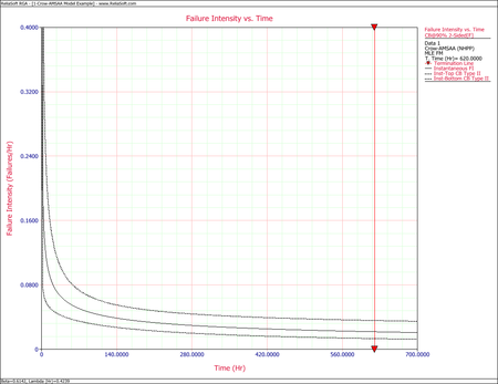
The following figures display plots of the Fisher Matrix confidence bounds for the cumulative and instantaneous failure intensity, respectively.
Crow Bounds
Given that the data is failure terminated, the Crow confidence bounds for the cumulative failure intensity at the 90% confidence level and for [math]\displaystyle{ T=620\,\! }[/math] hours are:
- [math]\displaystyle{ \begin{align} {{[{{\lambda }_{c}}(T)]}_{L}} = & \frac{\chi _{\tfrac{\alpha }{2},2N}^{2}}{2\cdot t} \\ = & \frac{29.787476}{2*620} \\ = & 0.02402 \\ {{[{{\lambda }_{c}}(T)]}_{U}} = & \frac{\chi _{1-\tfrac{\alpha }{2},2N}^{2}}{2\cdot t} \\ = & \frac{60.48089}{2*620} \\ = & 0.048775 \end{align}\,\! }[/math]
The Crow confidence bounds for the instantaneous failure intensity at the 90% confidence level and for [math]\displaystyle{ T=620\,\! }[/math] hours are calculated by first estimating the bounds on the instantaneous MTBF. Once these are calculated, take the inverse as shown below. Details on the confidence bounds for instantaneous MTBF are presented here.
- [math]\displaystyle{ \begin{align} {{[{{\lambda }_{i}}(t)]}_{L}} = & \frac{1}{{{[MTB{{F}_{i}}]}_{U}}} \\ = & \frac{1}{MTB{{F}_{i}}\cdot U} \\ = & 0.01179 \end{align}\,\! }[/math]
- [math]\displaystyle{ \begin{align} {{[{{\lambda }_{i}}(t)]}_{U}}= & \frac{1}{{{[MTB{{F}_{i}}]}_{L}}} \\ = & \frac{1}{MTB{{F}_{i}}\cdot L} \\ = & 0.03253 \end{align}\,\! }[/math]
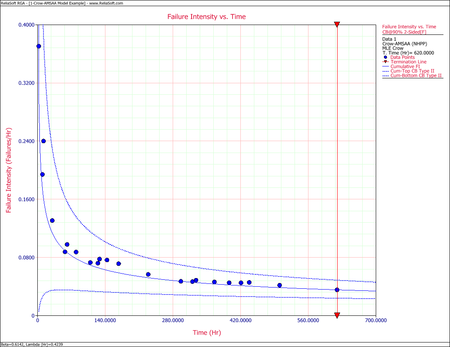
The following figures display plots of the Crow confidence bounds for the cumulative and instantaneous failure intensity, respectively.
Example - Confidence Bounds on MTBF
Calculate the confidence bounds on the cumulative and instantaneous MTBF for the data from the example given above.
Solution
Fisher Matrix Bounds
From the previous example:
- [math]\displaystyle{ \begin{align} Var(\hat{\lambda }) = & 0.13519969 \\ Var(\hat{\beta }) = & 0.017105343 \\ Cov(\hat{\beta },\hat{\lambda }) = & -0.046614609 \end{align}\,\! }[/math]
And for [math]\displaystyle{ T=620\,\! }[/math] hours, the partial derivatives of the cumulative and instantaneous MTBF are:
- [math]\displaystyle{ \begin{align} \frac{\partial {{m}_{c}}(T)}{\partial \beta }= & -\frac{1}{\hat{\lambda }}{{T}^{1-\hat{\beta }}}\ln T \\ = & -\frac{1}{0.4239}{{620}^{0.3858}}\ln 620 \\ = & -181.23135 \\ \frac{\partial {{m}_{c}}(T)}{\partial \lambda } = & -\frac{1}{{{\hat{\lambda }}^{2}}}{{T}^{1-\hat{\beta }}} \\ = & -\frac{1}{{{0.4239}^{2}}}{{620}^{0.3858}} \\ = & -66.493299 \\ \frac{\partial {{m}_{i}}(T)}{\partial \beta } = & -\frac{1}{\hat{\lambda }{{\hat{\beta }}^{2}}}{{T}^{1-\beta }}-\frac{1}{\hat{\lambda }\hat{\beta }}{{T}^{1-\hat{\beta }}}\ln T \\ = & -\frac{1}{0.4239\cdot {{0.6142}^{2}}}{{620}^{0.3858}}-\frac{1}{0.4239\cdot 0.6142}{{620}^{0.3858}}\ln 620 \\ = & -369.78634 \\ \frac{\partial {{m}_{i}}(T)}{\partial \lambda } = & -\frac{1}{{{\hat{\lambda }}^{2}}\hat{\beta }}{{T}^{1-\hat{\beta }}} \\ = & -\frac{1}{{{0.4239}^{2}}\cdot 0.6142}\cdot {{620}^{0.3858}} \\ = & -108.26001 \end{align}\,\! }[/math]
Therefore, the variances become:
- [math]\displaystyle{ \begin{align} Var({{\hat{m}}_{c}}(T)) = & {{\left( -181.23135 \right)}^{2}}\cdot 0.017105343+{{\left( -66.493299 \right)}^{2}}\cdot 0.13519969 \\ & -2\cdot \left( -181.23135 \right)\cdot \left( -66.493299 \right)\cdot 0.046614609 \\ = & 36.113376 \end{align}\,\! }[/math]
- [math]\displaystyle{ \begin{align} Var({{\hat{m}}_{i}}(T)) = & {{\left( -369.78634 \right)}^{2}}\cdot 0.017105343+{{\left( -108.26001 \right)}^{2}}\cdot 0.13519969 \\ & -2\cdot \left( -369.78634 \right)\cdot \left( -108.26001 \right)\cdot 0.046614609 \\ = & 191.33709 \end{align}\,\! }[/math]
So, at 90% confidence level and [math]\displaystyle{ T=620\,\! }[/math] hours, the Fisher Matrix confidence bounds are:
- [math]\displaystyle{ \begin{align} {{[{{m}_{c}}(T)]}_{L}} = & {{{\hat{m}}}_{c}}(t){{e}^{-{{z}_{\alpha }}\sqrt{Var({{{\hat{m}}}_{c}}(t))}/{{{\hat{m}}}_{c}}(t)}} \\ = & 19.84581 \\ {{[{{m}_{c}}(T)]}_{U}} = & {{{\hat{m}}}_{c}}(t){{e}^{{{z}_{\alpha }}\sqrt{Var({{{\hat{m}}}_{c}}(t))}/{{{\hat{m}}}_{c}}(t)}} \\ = & 40.01927 \end{align}\,\! }[/math]
- [math]\displaystyle{ \begin{align} {{[{{m}_{i}}(T)]}_{L}} = & {{{\hat{m}}}_{i}}(t){{e}^{-{{z}_{\alpha }}\sqrt{Var({{{\hat{m}}}_{i}}(t))}/{{{\hat{m}}}_{i}}(t)}} \\ = & 27.94261 \\ {{[{{m}_{i}}(T)]}_{U}} = & {{{\hat{m}}}_{i}}(t){{e}^{{{z}_{\alpha }}\sqrt{Var({{{\hat{m}}}_{i}}(t))}/{{{\hat{m}}}_{i}}(t)}} \\ = & 75.34193 \end{align}\,\! }[/math]
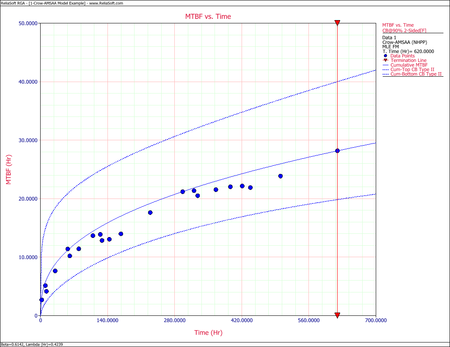
The following two figures show plots of the Fisher Matrix confidence bounds for the cumulative and instantaneous MTBFs.
Crow Bounds
The Crow confidence bounds for the cumulative MTBF and the instantaneous MTBF at the 90% confidence level and for [math]\displaystyle{ T=620\,\! }[/math] hours are:
- [math]\displaystyle{ \begin{align} {{[{{m}_{c}}(T)]}_{L}} = & \frac{1}{{{[{{\lambda }_{c}}(T)]}_{U}}} \\ = & 20.5023 \\ {{[{{m}_{c}}(T)]}_{U}} = & \frac{1}{{{[{{\lambda }_{c}}(T)]}_{L}}} \\ = & 41.6282 \end{align}\,\! }[/math]
- [math]\displaystyle{ \begin{align} {{[MTB{{F}_{i}}]}_{L}} = & MTB{{F}_{i}}\cdot {{\Pi }_{1}} \\ = & 30.7445 \\ {{[MTB{{F}_{i}}]}_{U}} = & MTB{{F}_{i}}\cdot {{\Pi }_{2}} \\ = & 84.7972 \end{align}\,\! }[/math]
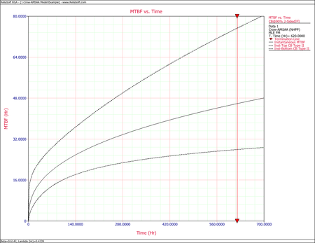
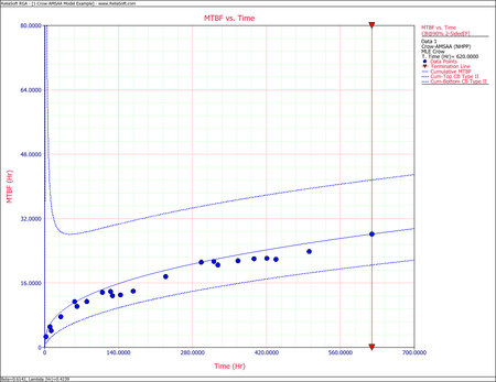
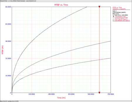
The figures below show plots of the Crow confidence bounds for the cumulative and instantaneous MTBF.
Confidence bounds can also be obtained on the parameters [math]\displaystyle{ \hat{\beta }\,\! }[/math] and [math]\displaystyle{ \hat{\lambda }\,\! }[/math]. For Fisher Matrix confidence bounds:
- [math]\displaystyle{ \begin{align} {{\beta }_{L}} = & \hat{\beta }{{e}^{{{z}_{\alpha }}\sqrt{Var(\hat{\beta })}/\hat{\beta }}} \\ = & 0.4325 \\ {{\beta }_{U}} = & \hat{\beta }{{e}^{-{{z}_{\alpha }}\sqrt{Var(\hat{\beta })}/\hat{\beta }}} \\ = & 0.8722 \end{align}\,\! }[/math]
and:
- [math]\displaystyle{ \begin{align} {{\lambda }_{L}} = & \hat{\lambda }{{e}^{{{z}_{\alpha }}\sqrt{Var(\hat{\lambda })}/\hat{\lambda }}} \\ = & 0.1016 \\ {{\lambda }_{U}} = & \hat{\lambda }{{e}^{-{{z}_{\alpha }}\sqrt{Var(\hat{\lambda })}/\hat{\lambda }}} \\ = & 1.7691 \end{align}\,\! }[/math]
For Crow confidence bounds:
- [math]\displaystyle{ \begin{align} {{\beta }_{L}}= & 0.4527 \\ {{\beta }_{U}}= & 0.9350 \end{align}\,\! }[/math]
and:
- [math]\displaystyle{ \begin{align} {{\lambda }_{L}}= & 0.2870 \\ {{\lambda }_{U}}= & 0.5827 \end{align}\,\! }[/math]


