Crow-AMSAA Discrete Model Grouped Data Example: Difference between revisions
mNo edit summary |
Lisa Hacker (talk | contribs) No edit summary |
||
| Line 1: | Line 1: | ||
<noinclude>{{Banner RGA Examples}} | <noinclude>{{Banner RGA Examples}} | ||
''This example appears in the [ | ''This example appears in the [https://help.reliasoft.com/reference/reliability_growth_and_repairable_system_analysis Reliability growth reference]''. | ||
</noinclude> | </noinclude> | ||
Latest revision as of 21:22, 18 September 2023
New format available! This reference is now available in a new format that offers faster page load, improved display for calculations and images and more targeted search.
As of January 2024, this Reliawiki page will not continue to be updated. Please update all links and bookmarks to the latest references at RGA examples and RGA reference examples.
This example appears in the Reliability growth reference.
The table below shows the number of failures of each interval of trials and the cumulative number of trials in each interval for a reliability growth test. For example, the first row indicates that for an interval of 14 trials, 5 failures occurred.
| Failures in Interval | Cumulative Trials |
|---|---|
| 5 | 14 |
| 3 | 33 |
| 4 | 48 |
| 0 | 52 |
| 1 | 53 |
| 0 | 57 |
| 1 | 58 |
| 0 | 62 |
| 1 | 63 |
| 0 | 67 |
| 1 | 68 |
Using the RGA software, the parameters of the Crow-AMSAA model are estimated as follows:
- [math]\displaystyle{ \hat{\beta }=0.7950\,\! }[/math]
and:
- [math]\displaystyle{ \hat{\lambda }=0.5588\,\! }[/math]
As we have seen, the Crow-AMSAA instantaneous failure intensity, [math]\displaystyle{ {{\lambda }_{i}}(T)\,\! }[/math], is defined as:
- [math]\displaystyle{ \begin{align} {{\lambda }_{i}}(T)=\lambda \beta {{T}^{\beta -1}},\text{with }T\gt 0,\text{ }\lambda \gt 0\text{ and }\beta \gt 0 \end{align}\,\! }[/math]
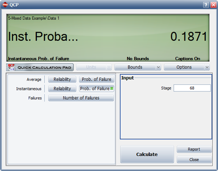
Using the parameter estimates, we can calculate the instantaneous unreliability at the end of the test, or [math]\displaystyle{ T=68.\,\! }[/math]
- [math]\displaystyle{ {{R}_{i}}(68)=0.5588\cdot 0.7950\cdot {{68}^{0.7950-1}}=0.1871\,\! }[/math]
This result that can be obtained from the Quick Calculation Pad (QCP), for [math]\displaystyle{ T=68,\,\! }[/math] as seen in the following picture.
The instantaneous reliability can then be calculated as:
- [math]\displaystyle{ \begin{align} {{R}_{inst}}=1-0.1871=0.8129 \end{align}\,\! }[/math]

