BlockSim Allocation Analysis Example: Difference between revisions
Lisa Hacker (talk | contribs) No edit summary |
Lisa Hacker (talk | contribs) No edit summary |
||
| (8 intermediate revisions by one other user not shown) | |||
| Line 1: | Line 1: | ||
<noinclude>{{Banner BlockSim Examples}} | <noinclude>{{Banner BlockSim Examples}} | ||
''This example also appears in the [ | ''This example also appears in the [https://help.reliasoft.com/reference/system_analysis System analysis reference]''.</noinclude> | ||
Consider a system consisting of three components connected reliability-wise in series. Assume the objective reliability for the system is 90% for a mission time of 100 hours. Five cases will be considered for the allocation problem. See [[Appendix_B:_References | | Consider a system consisting of three components connected reliability-wise in series. Assume the objective reliability for the system is 90% for a mission time of 100 hours. Five cases will be considered for the allocation problem. See Mettas [[Appendix_B:_References | [21]]]. | ||
<br> | <br> | ||
*'''Case 1''' - All three components are identical with times-to-failure that are described by a Weibull distribution with | *'''Case 1''' - All three components are identical with times-to-failure that are described by a Weibull distribution with <math>\beta = 1.318\,\!</math> and <math>\eta = 312\,\!</math> hours. All three components have the same feasibility value of Moderate (5).<br> | ||
*'''Case 2''' - Same as in Case 1, but Component 1 has a feasibility of Easy, Component 2 has a feasibility of Moderate and Component 3 has a feasibility of Hard.<br> | *'''Case 2''' - Same as in Case 1, but Component 1 has a feasibility of Easy, Component 2 has a feasibility of Moderate and Component 3 has a feasibility of Hard.<br> | ||
*'''Case 3''' - Component 1 has 70% reliability, Component 2 has 80% reliability and Component 3 has 90% reliability, all for a mission duration of 100 hours. All three components have the same feasibility of Easy.<br> | *'''Case 3''' - Component 1 has 70% reliability, Component 2 has 80% reliability and Component 3 has 90% reliability, all for a mission duration of 100 hours. All three components have the same feasibility of Easy.<br> | ||
| Line 10: | Line 10: | ||
*'''Case 5''' - Component 1 has 70% reliability and Hard feasibility, Component 2 has 80% reliability and Easy feasibility and Component 3 has 90% reliability and Moderate feasibility, all for a mission duration of 100 hours.<br> | *'''Case 5''' - Component 1 has 70% reliability and Hard feasibility, Component 2 has 80% reliability and Easy feasibility and Component 3 has 90% reliability and Moderate feasibility, all for a mission duration of 100 hours.<br> | ||
In all cases, the maximum achievable reliability, | In all cases, the maximum achievable reliability, <math>{{R}_{max,i}}\,\!</math>, for each component is 99.9% for a mission duration of 100 hours. | ||
'''Case 1''' - The reliability equation for Case 1 is: | '''Case 1''' - The reliability equation for Case 1 is: | ||
::<math>{{R}_{_{S}}}(t)={{R}_{1}}(t)\cdot {{R}_{2}}(t)\cdot {{R}_{3}}(t)</math> | ::<math>{{R}_{_{S}}}(t)={{R}_{1}}(t)\cdot {{R}_{2}}(t)\cdot {{R}_{3}}(t)\,\!</math> | ||
Thus, the equality desired is: | Thus, the equality desired is: | ||
::<math>0.90={{R}_{1}}(t=100)\cdot {{R}_{2}}(t=100)\cdot {{R}_{3}}(t=100)\ </math> | ::<math>0.90={{R}_{1}}(t=100)\cdot {{R}_{2}}(t=100)\cdot {{R}_{3}}(t=100)\,\!</math> | ||
where: | where: | ||
::<math>{{R}_{1,2,3}}={{e}^{-{{\left( \tfrac{t}{\eta } \right)}^{\beta }}}}</math> | ::<math>{{R}_{1,2,3}}={{e}^{-{{\left( \tfrac{t}{\eta } \right)}^{\beta }}}}\,\!</math> | ||
The cost or feasibility function is: | The cost or feasibility function is: | ||
::<math>{{C}_{T}}={{C}_{1}}({{R}_{1}})+{{C}_{2}}({{R}_{2}})+{{C}_{3}}({{R}_{3}})\ </math> | ::<math>{{C}_{T}}={{C}_{1}}({{R}_{1}})+{{C}_{2}}({{R}_{2}})+{{C}_{3}}({{R}_{3}})\,\!</math> | ||
where: | where: | ||
::<math>{{C}_{1,2,3}}({{R}_{1,2,3}})={{e}^{(1-f)\cdot \tfrac{{{R}_{i}}-{{R}_{\min ,i}}}{{{R}_{\max ,i}}-{{R}_{i}}}}}</math> | ::<math>{{C}_{1,2,3}}({{R}_{1,2,3}})={{e}^{(1-f)\cdot \tfrac{{{R}_{i}}-{{R}_{\min ,i}}}{{{R}_{\max ,i}}-{{R}_{i}}}}}\,\!</math> | ||
And where | And where <math>{{R}_{\max _{1,2,3}^{}}}=0.999\,\!</math> (arbitrarily set), <math>{{R}_{\min _{1,2,3}^{}}}\,\!</math> computed from the reliability function of each component at the time of interest, <math>t=100\,\!</math>, or: | ||
::<math>\begin{align} | ::<math>\begin{align} | ||
| Line 38: | Line 38: | ||
= & {{e}^{-{{\left( \tfrac{100}{312} \right)}^{1.318}}}} \\ | = & {{e}^{-{{\left( \tfrac{100}{312} \right)}^{1.318}}}} \\ | ||
= & 0.79995 | = & 0.79995 | ||
\end{align}</math> | \end{align}\,\!</math> | ||
And | And <math>f\,\!</math> obtained from: | ||
::<math>\begin{align} | ::<math>\begin{align} | ||
f= & \left( 1-\frac{5}{10} \right) \\ | f= & \left( 1-\frac{5}{10} \right) \\ | ||
= & 0.5 | = & 0.5 | ||
\end{align}</math> | \end{align}\,\!</math> | ||
The solution, | The solution, <math>{{R}_{{{O}_{i}}}}\,\!</math>, is the one that satisfies <math>0.90={{R}_{1}}(t=100)\cdot {{R}_{2}}(t=100)\cdot {{R}_{3}}(t=100)\,\!</math> while minimizing <math>{{C}_{T}}={{C}_{1}}({{R}_{1}})+{{C}_{2}}({{R}_{2}})+{{C}_{3}}({{R}_{3}})\,\!</math>. In this case (and since all the components are identical), the target reliability is found to be: | ||
::<math>{{R}_{{{O}_{i}}}}(t=100)=0.9655</math> | ::<math>{{R}_{{{O}_{i}}}}(t=100)=0.9655\,\!</math> | ||
The following figure shows the optimization results from BlockSim. | The following figure shows the optimization results from BlockSim. | ||
[[Image:6.17.png|center|700px|Optimization results for Case 1.]] | [[Image:6.17.png|center|700px|Optimization results for Case 1.|link=]] | ||
Based on this, each component's reliability should be at least 96.55% at 100 hours in order for the system's reliability to be 90% at 100 hours. Note the column labeled "Equivalent Parallel Units" which represents the number of redundant units that would be required to bring that particular component up to the recommended reliability. In the case where the fault tolerance approach is to be implemented, the "Equivalent Parallel Units" value should be rounded up to an integer. Therefore, some manipulation by the engineer is required in order to ensure that the chosen integer values will yield the required system reliability goal (or exceed it). In addition, further cost analysis should be performed in order to account for the costs of adding redundancy to the system. | Based on this, each component's reliability should be at least 96.55% at 100 hours in order for the system's reliability to be 90% at 100 hours. Note the column labeled "Equivalent Parallel Units" which represents the number of redundant units that would be required to bring that particular component up to the recommended reliability. In the case where the fault tolerance approach is to be implemented, the "Equivalent Parallel Units" value should be rounded up to an integer. Therefore, some manipulation by the engineer is required in order to ensure that the chosen integer values will yield the required system reliability goal (or exceed it). In addition, further cost analysis should be performed in order to account for the costs of adding redundancy to the system. | ||
Additionally, and when the results have been obtained, the engineer may wish to re-scale the components based on their distribution parameters instead of the fixed reliability value. | Additionally, and when the results have been obtained, the engineer may wish to re-scale the components based on their distribution parameters instead of the fixed reliability value. In the case of these components, one may wish to re-scale the scale parameter of the distribution, <math>\eta \,\!</math>, for the components, or: | ||
::<math>\begin{align} | ::<math>\begin{align} | ||
0.9655= & {{e}^{-{{\left( \tfrac{t}{\eta } \right)}^{\beta }}}} \\ | 0.9655= & {{e}^{-{{\left( \tfrac{t}{\eta } \right)}^{\beta }}}} \\ | ||
0.9655= & {{e}^{-{{\left( \tfrac{100}{\eta } \right)}^{1.318}}}} | 0.9655= & {{e}^{-{{\left( \tfrac{100}{\eta } \right)}^{1.318}}}} | ||
\end{align}</math> | \end{align}\,\!</math> | ||
Which yields: | Which yields: | ||
::<math>{{\eta }_{{{O}_{i}}}}=1269.48</math> | ::<math>{{\eta }_{{{O}_{i}}}}=1269.48\,\!</math> | ||
The Quick Parameter Estimator (QPE) in BlockSim can also be used for this, as shown below. | The Quick Parameter Estimator (QPE) in BlockSim can also be used for this, as shown below. | ||
[[Image:BS6.18.png|center| | [[Image:BS6.18.png|center|600px|BlockSim's Quick Parameter Estimator (QPE) used to determine a new eta based on the newly determined reliability target|link=]] | ||
The results from the other cases can be obtained in a similar fashion. The results for Cases 1 through 5 are summarized next. | The results from the other cases can be obtained in a similar fashion. The results for Cases 1 through 5 are summarized next. | ||
| Line 79: | Line 79: | ||
Component 2 & \text{0}\text{.9655} & \text{0}\text{.9633} & \text{0}\text{.9649} & \text{0}\text{.9553} & \text{0}\text{.9884} \\ | Component 2 & \text{0}\text{.9655} & \text{0}\text{.9633} & \text{0}\text{.9649} & \text{0}\text{.9553} & \text{0}\text{.9884} \\ | ||
Component 3 & \text{0}\text{.9655} & \text{0}\text{.9463} & \text{0}\text{.9765} & \text{0}\text{.9624} & \text{0}\text{.9797} \\ | Component 3 & \text{0}\text{.9655} & \text{0}\text{.9463} & \text{0}\text{.9765} & \text{0}\text{.9624} & \text{0}\text{.9797} \\ | ||
\end{matrix}</math> | \end{matrix}\,\!</math> | ||
'''Case 2''' - It can be seen that the highest reliability was allocated to Component 1 with the Easy feasibility. The lowest reliability was assigned to Component 3 with the Hard feasibility. This makes sense in that an optimized reliability scheme will call for the greatest reliability changes in those components that are the easiest to change. | '''Case 2''' - It can be seen that the highest reliability was allocated to Component 1 with the Easy feasibility. The lowest reliability was assigned to Component 3 with the Hard feasibility. This makes sense in that an optimized reliability scheme will call for the greatest reliability changes in those components that are the easiest to change. | ||
| Line 89: | Line 89: | ||
The next figure shows the reliability importance for each component, where it can be seen that Component 1 has the greatest reliability importance and Component 3 has the smallest (this reliability importance also applies in Cases 4 and 5). This indicates that the reliability of Component 1 should be significantly increased because it has the biggest impact on the overall system reliability. | The next figure shows the reliability importance for each component, where it can be seen that Component 1 has the greatest reliability importance and Component 3 has the smallest (this reliability importance also applies in Cases 4 and 5). This indicates that the reliability of Component 1 should be significantly increased because it has the biggest impact on the overall system reliability. | ||
[[Image:6.19.png|center| | [[Image:6.19.png|center|500px|Reliability importance for Cases 3, 4, and 5.|link=]] | ||
In addition, each component's cost function in Case 3 also depends on the difference between each component's initial reliability and its corresponding maximum achievable reliability. (In Cases 1 and 2 this was not an issue because the components were identical.) The greater this difference, the greater the cost of improving the reliability of a particular component relative to the other two components. This difference between the initial reliability of a component and its maximum achievable reliability is called the range of improvement for that component. Since all three components have the same maximum achievable reliability, Component 1, with the largest range for improvement, is the most cost efficient component to improve. The improvement ranges for all three components are illustrated in the next figure. At the same time, however, there is a reliability value between the initial and the maximum achievable reliability beyond which it becomes cost prohibitive to improve any further. This reliability value is dictated by the feasibility value. From the table of results, it can be seen that in Case 3 there was a 25.52% improvement for Component 1, 16.49% for Component 2 and 7.65% for Component 3. | In addition, each component's cost function in Case 3 also depends on the difference between each component's initial reliability and its corresponding maximum achievable reliability. (In Cases 1 and 2 this was not an issue because the components were identical.) The greater this difference, the greater the cost of improving the reliability of a particular component relative to the other two components. This difference between the initial reliability of a component and its maximum achievable reliability is called the range of improvement for that component. Since all three components have the same maximum achievable reliability, Component 1, with the largest range for improvement, is the most cost efficient component to improve. The improvement ranges for all three components are illustrated in the next figure. At the same time, however, there is a reliability value between the initial and the maximum achievable reliability beyond which it becomes cost prohibitive to improve any further. This reliability value is dictated by the feasibility value. From the table of results, it can be seen that in Case 3 there was a 25.52% improvement for Component 1, 16.49% for Component 2 and 7.65% for Component 3. | ||
[[Image:6.20.png|center| | [[Image:6.20.png|center|350px|Range of improvement for each component for Cases 3, 4, and 5.|link=]] | ||
'''Case 4''' - As opposed to Case 3, Component 1 was assigned an even greater increase of 27.9%, with Components 2 and 3 receiving lesser increases than in Case 3, of 15.53% and 6.24% respectively. This is due to the fact that Component 1 has an Easy feasibility and Component 3 has a Hard feasibility, which means that it is more difficult to increase the reliability of Component 3 than to increase the reliability of Component 1. | '''Case 4''' - As opposed to Case 3, Component 1 was assigned an even greater increase of 27.9%, with Components 2 and 3 receiving lesser increases than in Case 3, of 15.53% and 6.24% respectively. This is due to the fact that Component 1 has an Easy feasibility and Component 3 has a Hard feasibility, which means that it is more difficult to increase the reliability of Component 3 than to increase the reliability of Component 1. | ||
'''Case 5''' - The feasibility values here are reversed with Component 1 having a Hard feasibility and Component 3 an Easy feasibility. The recommended increase in Component 1's reliability is less compared to its increase for Cases 3 and 4. Note, however, that Components 2 and 3 still received a smaller increase in reliability than Component 1 because their ranges of improvement are smaller. In other words, Component 3 was assigned the smallest increase in reliability in Cases 3, 4 and 5 because its initial reliability is very close to its maximum achievable reliability. | '''Case 5''' - The feasibility values here are reversed with Component 1 having a Hard feasibility and Component 3 an Easy feasibility. The recommended increase in Component 1's reliability is less compared to its increase for Cases 3 and 4. Note, however, that Components 2 and 3 still received a smaller increase in reliability than Component 1 because their ranges of improvement are smaller. In other words, Component 3 was assigned the smallest increase in reliability in Cases 3, 4 and 5 because its initial reliability is very close to its maximum achievable reliability. | ||
Latest revision as of 20:56, 18 September 2023
New format available! This reference is now available in a new format that offers faster page load, improved display for calculations and images and more targeted search.
As of January 2024, this Reliawiki page will not continue to be updated. Please update all links and bookmarks to the latest references at BlockSim examples and BlockSim reference examples.
This example also appears in the System analysis reference.
Consider a system consisting of three components connected reliability-wise in series. Assume the objective reliability for the system is 90% for a mission time of 100 hours. Five cases will be considered for the allocation problem. See Mettas [21].
- Case 1 - All three components are identical with times-to-failure that are described by a Weibull distribution with [math]\displaystyle{ \beta = 1.318\,\! }[/math] and [math]\displaystyle{ \eta = 312\,\! }[/math] hours. All three components have the same feasibility value of Moderate (5).
- Case 2 - Same as in Case 1, but Component 1 has a feasibility of Easy, Component 2 has a feasibility of Moderate and Component 3 has a feasibility of Hard.
- Case 3 - Component 1 has 70% reliability, Component 2 has 80% reliability and Component 3 has 90% reliability, all for a mission duration of 100 hours. All three components have the same feasibility of Easy.
- Case 4 - Component 1 has 70% reliability and Easy feasibility, Component 2 has 80% reliability and Moderate feasibility, and Component 3 has 90% reliability and Hard feasibility, all for a mission duration of 100 hours.
- Case 5 - Component 1 has 70% reliability and Hard feasibility, Component 2 has 80% reliability and Easy feasibility and Component 3 has 90% reliability and Moderate feasibility, all for a mission duration of 100 hours.
In all cases, the maximum achievable reliability, [math]\displaystyle{ {{R}_{max,i}}\,\! }[/math], for each component is 99.9% for a mission duration of 100 hours.
Case 1 - The reliability equation for Case 1 is:
- [math]\displaystyle{ {{R}_{_{S}}}(t)={{R}_{1}}(t)\cdot {{R}_{2}}(t)\cdot {{R}_{3}}(t)\,\! }[/math]
Thus, the equality desired is:
- [math]\displaystyle{ 0.90={{R}_{1}}(t=100)\cdot {{R}_{2}}(t=100)\cdot {{R}_{3}}(t=100)\,\! }[/math]
where:
- [math]\displaystyle{ {{R}_{1,2,3}}={{e}^{-{{\left( \tfrac{t}{\eta } \right)}^{\beta }}}}\,\! }[/math]
The cost or feasibility function is:
- [math]\displaystyle{ {{C}_{T}}={{C}_{1}}({{R}_{1}})+{{C}_{2}}({{R}_{2}})+{{C}_{3}}({{R}_{3}})\,\! }[/math]
where:
- [math]\displaystyle{ {{C}_{1,2,3}}({{R}_{1,2,3}})={{e}^{(1-f)\cdot \tfrac{{{R}_{i}}-{{R}_{\min ,i}}}{{{R}_{\max ,i}}-{{R}_{i}}}}}\,\! }[/math]
And where [math]\displaystyle{ {{R}_{\max _{1,2,3}^{}}}=0.999\,\! }[/math] (arbitrarily set), [math]\displaystyle{ {{R}_{\min _{1,2,3}^{}}}\,\! }[/math] computed from the reliability function of each component at the time of interest, [math]\displaystyle{ t=100\,\! }[/math], or:
- [math]\displaystyle{ \begin{align} {{R}_{\min _{1,2,3}^{}}}= & {{e}^{-{{\left( \tfrac{t}{\eta } \right)}^{\beta }}}} \\ = & {{e}^{-{{\left( \tfrac{100}{312} \right)}^{1.318}}}} \\ = & 0.79995 \end{align}\,\! }[/math]
And [math]\displaystyle{ f\,\! }[/math] obtained from:
- [math]\displaystyle{ \begin{align} f= & \left( 1-\frac{5}{10} \right) \\ = & 0.5 \end{align}\,\! }[/math]
The solution, [math]\displaystyle{ {{R}_{{{O}_{i}}}}\,\! }[/math], is the one that satisfies [math]\displaystyle{ 0.90={{R}_{1}}(t=100)\cdot {{R}_{2}}(t=100)\cdot {{R}_{3}}(t=100)\,\! }[/math] while minimizing [math]\displaystyle{ {{C}_{T}}={{C}_{1}}({{R}_{1}})+{{C}_{2}}({{R}_{2}})+{{C}_{3}}({{R}_{3}})\,\! }[/math]. In this case (and since all the components are identical), the target reliability is found to be:
- [math]\displaystyle{ {{R}_{{{O}_{i}}}}(t=100)=0.9655\,\! }[/math]
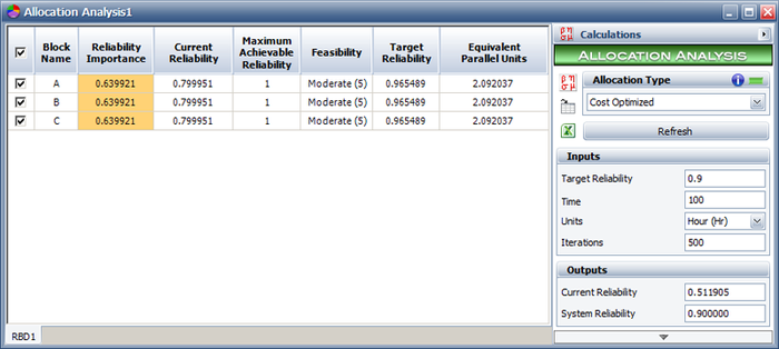
The following figure shows the optimization results from BlockSim.

Based on this, each component's reliability should be at least 96.55% at 100 hours in order for the system's reliability to be 90% at 100 hours. Note the column labeled "Equivalent Parallel Units" which represents the number of redundant units that would be required to bring that particular component up to the recommended reliability. In the case where the fault tolerance approach is to be implemented, the "Equivalent Parallel Units" value should be rounded up to an integer. Therefore, some manipulation by the engineer is required in order to ensure that the chosen integer values will yield the required system reliability goal (or exceed it). In addition, further cost analysis should be performed in order to account for the costs of adding redundancy to the system.
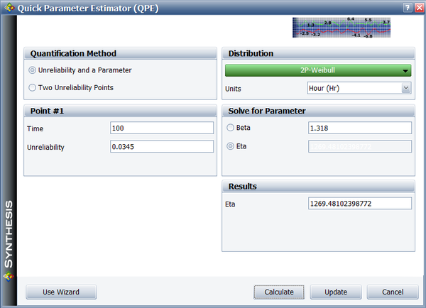
Additionally, and when the results have been obtained, the engineer may wish to re-scale the components based on their distribution parameters instead of the fixed reliability value. In the case of these components, one may wish to re-scale the scale parameter of the distribution, [math]\displaystyle{ \eta \,\! }[/math], for the components, or:
- [math]\displaystyle{ \begin{align} 0.9655= & {{e}^{-{{\left( \tfrac{t}{\eta } \right)}^{\beta }}}} \\ 0.9655= & {{e}^{-{{\left( \tfrac{100}{\eta } \right)}^{1.318}}}} \end{align}\,\! }[/math]
Which yields:
- [math]\displaystyle{ {{\eta }_{{{O}_{i}}}}=1269.48\,\! }[/math]
The Quick Parameter Estimator (QPE) in BlockSim can also be used for this, as shown below.

The results from the other cases can be obtained in a similar fashion. The results for Cases 1 through 5 are summarized next.
- [math]\displaystyle{ \begin{matrix} {} & Case 1 & Case 2 & Case 3 & Case 4 & Case 5 \\ Component 1 & \text{0}\text{.9655} & \text{0}\text{.9874} & \text{0}\text{.9552} & \text{0}\text{.9790} & \text{0}\text{.9295} \\ Component 2 & \text{0}\text{.9655} & \text{0}\text{.9633} & \text{0}\text{.9649} & \text{0}\text{.9553} & \text{0}\text{.9884} \\ Component 3 & \text{0}\text{.9655} & \text{0}\text{.9463} & \text{0}\text{.9765} & \text{0}\text{.9624} & \text{0}\text{.9797} \\ \end{matrix}\,\! }[/math]
Case 2 - It can be seen that the highest reliability was allocated to Component 1 with the Easy feasibility. The lowest reliability was assigned to Component 3 with the Hard feasibility. This makes sense in that an optimized reliability scheme will call for the greatest reliability changes in those components that are the easiest to change.
Case 3 - The components were different but had the same feasibility values.
In other words, all three components have the same opportunity for improvement. This case differs from Cases 1 and 2 since there are two factors, not present previously, that will affect the outcome of the allocation in this case. First, each component in this case has a different reliability importance (impact of a component on the system's reliability); whereas in Cases 1 and 2, all three components were identical and had the same reliability importance.
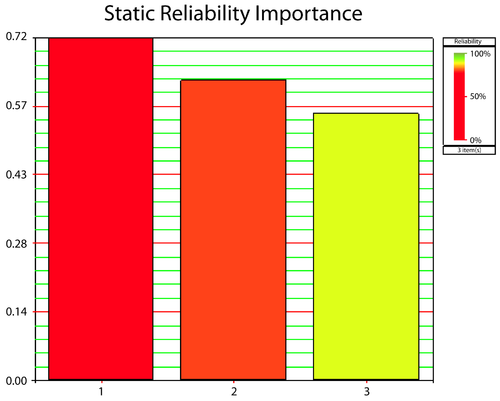
The next figure shows the reliability importance for each component, where it can be seen that Component 1 has the greatest reliability importance and Component 3 has the smallest (this reliability importance also applies in Cases 4 and 5). This indicates that the reliability of Component 1 should be significantly increased because it has the biggest impact on the overall system reliability.

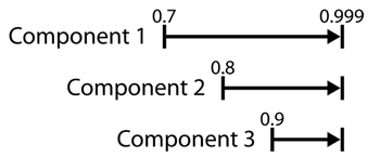
In addition, each component's cost function in Case 3 also depends on the difference between each component's initial reliability and its corresponding maximum achievable reliability. (In Cases 1 and 2 this was not an issue because the components were identical.) The greater this difference, the greater the cost of improving the reliability of a particular component relative to the other two components. This difference between the initial reliability of a component and its maximum achievable reliability is called the range of improvement for that component. Since all three components have the same maximum achievable reliability, Component 1, with the largest range for improvement, is the most cost efficient component to improve. The improvement ranges for all three components are illustrated in the next figure. At the same time, however, there is a reliability value between the initial and the maximum achievable reliability beyond which it becomes cost prohibitive to improve any further. This reliability value is dictated by the feasibility value. From the table of results, it can be seen that in Case 3 there was a 25.52% improvement for Component 1, 16.49% for Component 2 and 7.65% for Component 3.

Case 4 - As opposed to Case 3, Component 1 was assigned an even greater increase of 27.9%, with Components 2 and 3 receiving lesser increases than in Case 3, of 15.53% and 6.24% respectively. This is due to the fact that Component 1 has an Easy feasibility and Component 3 has a Hard feasibility, which means that it is more difficult to increase the reliability of Component 3 than to increase the reliability of Component 1.
Case 5 - The feasibility values here are reversed with Component 1 having a Hard feasibility and Component 3 an Easy feasibility. The recommended increase in Component 1's reliability is less compared to its increase for Cases 3 and 4. Note, however, that Components 2 and 3 still received a smaller increase in reliability than Component 1 because their ranges of improvement are smaller. In other words, Component 3 was assigned the smallest increase in reliability in Cases 3, 4 and 5 because its initial reliability is very close to its maximum achievable reliability.
