General Log-Linear Relationship Example: Difference between revisions
No edit summary |
Lisa Hacker (talk | contribs) No edit summary |
||
| (7 intermediate revisions by 4 users not shown) | |||
| Line 1: | Line 1: | ||
<noinclude>{{Banner_ALTA_Examples}} | <noinclude>{{Banner_ALTA_Examples}} | ||
</noinclude>Consider the data summarized in the following tables. These data illustrate a typical three-stress type accelerated test. | ''This example appears in the [https://help.reliasoft.com/reference/accelerated_life_testing_data_analysis Accelerated life testing reference].'' | ||
</noinclude> | |||
Consider the data summarized in the following tables. These data illustrate a typical three-stress type accelerated test. | |||
<center>Stress Profile Summary</center> | <center>Stress Profile Summary</center> | ||
| Line 7: | Line 10: | ||
<center>Failure Data</center> | <center>Failure Data</center> | ||
[[Image:ALTA11t2.png|center| | [[Image:ALTA11t2.png|center|550px|]] | ||
The data in the second table are analyzed assuming a Weibull distribution, an Arrhenius life-stress relationship for temperature and an inverse power life-stress relationship for voltage. No transformation is performed on the operation type. The operation type variable is treated as an indicator variable that takes a discrete value of 0 for an on/off operation and 1 for a continuous operation. The following figure shows the stress types and their transformations in ALTA. | |||
[[Image:StressTransformation.gif|center|450px|]] | [[Image:StressTransformation.gif|center|450px|]] | ||
| Line 15: | Line 19: | ||
The GLL relationship then becomes: | The GLL relationship then becomes: | ||
::<math>\eta ={{e}^{{{\alpha }_{0}}+{{\alpha }_{1}}\tfrac{1}{{{V}_{1}}}+{{\alpha }_{2}}\ln ({{V}_{2}})+{{\alpha }_{3}}{{V}_{3}}}}</math> | ::<math>\eta ={{e}^{{{\alpha }_{0}}+{{\alpha }_{1}}\tfrac{1}{{{V}_{1}}}+{{\alpha }_{2}}\ln ({{V}_{2}})+{{\alpha }_{3}}{{V}_{3}}}}\,\!</math> | ||
The resulting relationship after performing these transformations is: | The resulting relationship after performing these transformations is: | ||
| Line 21: | Line 25: | ||
::<math>\begin{align} | ::<math>\begin{align} | ||
& \eta = & {{e}^{{{\alpha }_{0}}}}{{e}^{{{\alpha }_{1}}\tfrac{1}{{{V}_{1}}}}}{{e}^{{{\alpha }_{2}}\ln ({{V}_{2}})}}{{e}^{{{\alpha }_{3}}{{V}_{3}}}} =\ & {{e}^{{{\alpha }_{0}}}}{{e}^{{{\alpha }_{1}}\tfrac{1}{{{V}_{1}}}}}V_{2}^{{{\alpha }_{2}}}{{e}^{{{\alpha }_{3}}{{V}_{3}}}} | & \eta = & {{e}^{{{\alpha }_{0}}}}{{e}^{{{\alpha }_{1}}\tfrac{1}{{{V}_{1}}}}}{{e}^{{{\alpha }_{2}}\ln ({{V}_{2}})}}{{e}^{{{\alpha }_{3}}{{V}_{3}}}} =\ & {{e}^{{{\alpha }_{0}}}}{{e}^{{{\alpha }_{1}}\tfrac{1}{{{V}_{1}}}}}V_{2}^{{{\alpha }_{2}}}{{e}^{{{\alpha }_{3}}{{V}_{3}}}} | ||
\end{align}</math> | \end{align}\,\!</math> | ||
Therefore, the parameter | Therefore, the parameter <math>B\,\!</math> of the Arrhenius relationship is equal to the log-linear coefficient <math>{{\alpha }_{1}}\,\!</math>, and the parameter <math>n\,\!</math> of the inverse power relationship is equal to (<math>-{{\alpha}_{2}}\,\!</math>). Therefore <math>\eta \,\!</math> can also be written as: | ||
::<math>\eta ={{e}^{{{\alpha }_{0}}}}{{e}^{\tfrac{B}{{{V}_{1}}}}}V_{2}^{n}{{e}^{{{\alpha }_{3}}{{V}_{3}}}}</math> | ::<math>\eta ={{e}^{{{\alpha }_{0}}}}{{e}^{\tfrac{B}{{{V}_{1}}}}}V_{2}^{n}{{e}^{{{\alpha }_{3}}{{V}_{3}}}}\,\!</math> | ||
The activation energy of the Arrhenius relationship can be calculated by multiplying B with Boltzmann's constant. | The activation energy of the Arrhenius relationship can be calculated by multiplying B with Boltzmann's constant. | ||
| Line 32: | Line 36: | ||
::<math>\begin{align} | ::<math>\begin{align} | ||
\beta = & 3.7483;\text{ }{{\alpha }_{0}}=-6.0220;\text{ }{{\alpha }_{1}}=5776.9341 \\ | \beta = & 3.7483;\text{ }{{\alpha }_{0}} = -6.0220;\text{ }{{\alpha }_{1}} = 5776.9341; \\ | ||
{{\alpha }_{2}}= & -1.4340;\text{ }{{\alpha }_{3}}=0.6242. | {{\alpha }_{2}} = & -1.4340;\text{ }{{\alpha }_{3}} = 0.6242. | ||
\end{align}</math> | \end{align}\,\!</math> | ||
Once the parameters are estimated, further analysis on the data can be performed. First, using ALTA, a Weibull probability plot of the data can be obtained, as shown next. | Once the parameters are estimated, further analysis on the data can be performed. First, using ALTA, a Weibull probability plot of the data can be obtained, as shown next. | ||
[[Image:ALTA11.1.gif|center|600px|Weibull probability plot for all covariates.]] | [[Image:ALTA11.1.gif|center|600px|Weibull probability plot for all covariates.]] | ||
Several types of information about the model as well as the data can be obtained from a probability plot. For example, the choice of an underlying distribution and the assumption of a common slope (shape parameter) can be examined. In this example, the linearity of the data supports the use of the Weibull distribution. In addition, the data appear parallel on this plot, therefore reinforcing the assumption of a common beta. Further statistical analysis can and should be performed for these purposes as well. | Several types of information about the model as well as the data can be obtained from a probability plot. For example, the choice of an underlying distribution and the assumption of a common slope (shape parameter) can be examined. In this example, the linearity of the data supports the use of the Weibull distribution. In addition, the data appear parallel on this plot, therefore reinforcing the assumption of a common beta. Further statistical analysis can and should be performed for these purposes as well. | ||
The Life vs. Stress plot is a very common plot for the analysis of accelerated data. Life vs. Stress plots can be very useful in assessing the effect of each stress on a product's failure. In this case, since the life is a function of three stresses, three different plots can be created. Such plots are created by holding two of the stresses constant at the desired use level, and varying the remaining one. The use stress levels for this example are 328K for temperature and 10V for voltage. For the operation type, a decision has to be made by the engineers as to whether they implement on/off or continuous operation. The next two figures display the effects of temperature and voltage on the life of the product. | |||
The Life vs. Stress plot is a very common plot for the analysis of accelerated data. Life vs. Stress plots can be very useful in assessing the effect of each stress on a product's failure. In this case, since the life is a function of three stresses, three different plots can be created. Such plots are created by holding two of the stresses constant at the desired use level, and varying the remaining one. The use stress levels for this example are 328K for temperature and 10V for voltage. For the operation type, a decision has to be made by the engineers as to whether they implement an on/off or continuous operation. The next two figures display the effects of temperature and voltage on the life of the product. | |||
[[Image:ALTA11.2.gif|center|600px|Effects of temperature on life.]] | [[Image:ALTA11.2.gif|center|600px|Effects of temperature on life.]] | ||
| Line 48: | Line 56: | ||
[[Image:ALTA11.3.gif|center|600px|Effects of voltage on life.]] | [[Image:ALTA11.3.gif|center|600px|Effects of voltage on life.]] | ||
The effects of the two different operation types on life can be observed in the next figure. It can be seen that the on/off cycling has a greater effect on the life of the product in terms of accelerating failure than the continuous operation. In other words, a higher reliability can be achieved by running the product continuously. | The effects of the two different operation types on life can be observed in the next figure. It can be seen that the on/off cycling has a greater effect on the life of the product in terms of accelerating failure than the continuous operation. In other words, a higher reliability can be achieved by running the product continuously. | ||
[[Image:ALTA11.4.gif|center|600px|Effect of operation type on life.]] | [[Image:ALTA11.4.gif|center|600px|Effect of operation type on life.]] | ||
Latest revision as of 19:03, 18 September 2023
New format available! This reference is now available in a new format that offers faster page load, improved display for calculations and images and more targeted search.
As of January 2024, this Reliawiki page will not continue to be updated. Please update all links and bookmarks to the latest references at ALTA examples and ALTA reference examples.
This example appears in the Accelerated life testing reference.
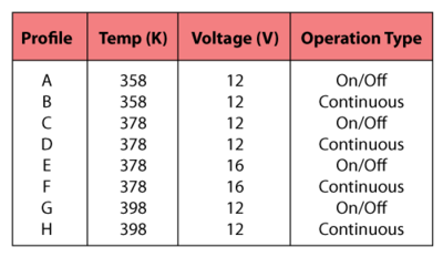
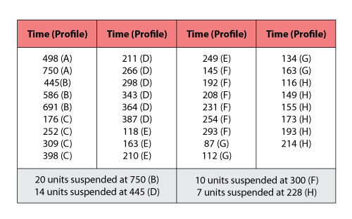
Consider the data summarized in the following tables. These data illustrate a typical three-stress type accelerated test.
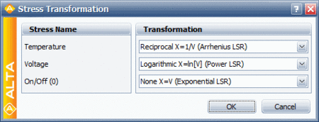
The data in the second table are analyzed assuming a Weibull distribution, an Arrhenius life-stress relationship for temperature and an inverse power life-stress relationship for voltage. No transformation is performed on the operation type. The operation type variable is treated as an indicator variable that takes a discrete value of 0 for an on/off operation and 1 for a continuous operation. The following figure shows the stress types and their transformations in ALTA.
The GLL relationship then becomes:
- [math]\displaystyle{ \eta ={{e}^{{{\alpha }_{0}}+{{\alpha }_{1}}\tfrac{1}{{{V}_{1}}}+{{\alpha }_{2}}\ln ({{V}_{2}})+{{\alpha }_{3}}{{V}_{3}}}}\,\! }[/math]
The resulting relationship after performing these transformations is:
- [math]\displaystyle{ \begin{align} & \eta = & {{e}^{{{\alpha }_{0}}}}{{e}^{{{\alpha }_{1}}\tfrac{1}{{{V}_{1}}}}}{{e}^{{{\alpha }_{2}}\ln ({{V}_{2}})}}{{e}^{{{\alpha }_{3}}{{V}_{3}}}} =\ & {{e}^{{{\alpha }_{0}}}}{{e}^{{{\alpha }_{1}}\tfrac{1}{{{V}_{1}}}}}V_{2}^{{{\alpha }_{2}}}{{e}^{{{\alpha }_{3}}{{V}_{3}}}} \end{align}\,\! }[/math]
Therefore, the parameter [math]\displaystyle{ B\,\! }[/math] of the Arrhenius relationship is equal to the log-linear coefficient [math]\displaystyle{ {{\alpha }_{1}}\,\! }[/math], and the parameter [math]\displaystyle{ n\,\! }[/math] of the inverse power relationship is equal to ([math]\displaystyle{ -{{\alpha}_{2}}\,\! }[/math]). Therefore [math]\displaystyle{ \eta \,\! }[/math] can also be written as:
- [math]\displaystyle{ \eta ={{e}^{{{\alpha }_{0}}}}{{e}^{\tfrac{B}{{{V}_{1}}}}}V_{2}^{n}{{e}^{{{\alpha }_{3}}{{V}_{3}}}}\,\! }[/math]
The activation energy of the Arrhenius relationship can be calculated by multiplying B with Boltzmann's constant.
The best fit values for the parameters in this case are:
- [math]\displaystyle{ \begin{align} \beta = & 3.7483;\text{ }{{\alpha }_{0}} = -6.0220;\text{ }{{\alpha }_{1}} = 5776.9341; \\ {{\alpha }_{2}} = & -1.4340;\text{ }{{\alpha }_{3}} = 0.6242. \end{align}\,\! }[/math]
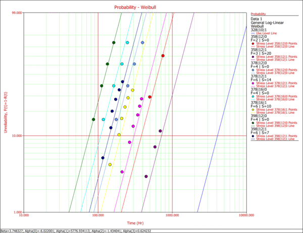
Once the parameters are estimated, further analysis on the data can be performed. First, using ALTA, a Weibull probability plot of the data can be obtained, as shown next.
Several types of information about the model as well as the data can be obtained from a probability plot. For example, the choice of an underlying distribution and the assumption of a common slope (shape parameter) can be examined. In this example, the linearity of the data supports the use of the Weibull distribution. In addition, the data appear parallel on this plot, therefore reinforcing the assumption of a common beta. Further statistical analysis can and should be performed for these purposes as well.
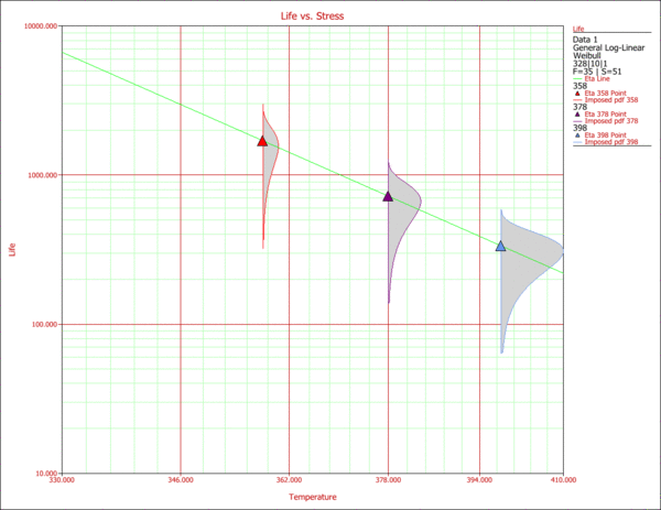
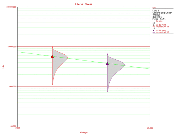
The Life vs. Stress plot is a very common plot for the analysis of accelerated data. Life vs. Stress plots can be very useful in assessing the effect of each stress on a product's failure. In this case, since the life is a function of three stresses, three different plots can be created. Such plots are created by holding two of the stresses constant at the desired use level, and varying the remaining one. The use stress levels for this example are 328K for temperature and 10V for voltage. For the operation type, a decision has to be made by the engineers as to whether they implement an on/off or continuous operation. The next two figures display the effects of temperature and voltage on the life of the product.
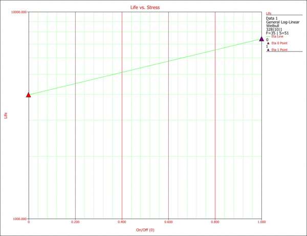
The effects of the two different operation types on life can be observed in the next figure. It can be seen that the on/off cycling has a greater effect on the life of the product in terms of accelerating failure than the continuous operation. In other words, a higher reliability can be achieved by running the product continuously.

