Simulation Based Bounds Example: Difference between revisions
Kate Racaza (talk | contribs) No edit summary |
Lisa Hacker (talk | contribs) No edit summary |
||
| (3 intermediate revisions by 2 users not shown) | |||
| Line 1: | Line 1: | ||
<noinclude>{{Banner Weibull Examples}} | <noinclude>{{Banner Weibull Examples}} | ||
''This example appears in the [[ | ''This example appears in the [https://help.reliasoft.com/reference/life_data_analysis Life data analysis reference] and [https://help.reliasoft.com/reference/accelerated_life_testing_data_analysis Accelerated life testing reference].'' | ||
</noinclude>'''Comparing Parameter Estimation Methods Using Simulation Based Bounds''' | </noinclude>'''Comparing Parameter Estimation Methods Using Simulation Based Bounds''' | ||
The purpose of this example is to determine the best parameter estimation method for a sample of ten units with complete time-to-failure data for each unit (i.e., no censoring). The data set follows a Weibull distribution with <math>\beta =2</math> and <math>\eta =100</math> | The purpose of this example is to determine the best parameter estimation method for a sample of ten units with complete time-to-failure data for each unit (i.e., no censoring). The data set follows a Weibull distribution with <math>\beta =2\,\!</math> and <math>\eta =100\,\!</math> hours. | ||
The confidence bounds for the data set could be obtained by using [[Weibull++ SimuMatic|'''Weibull++''''s SimuMatic]] utility. To obtain the results, use the following settings in SimuMatic. | The confidence bounds for the data set could be obtained by using [[Weibull++ SimuMatic|'''Weibull++''''s SimuMatic]] utility. To obtain the results, use the following settings in SimuMatic. | ||
:# On the Main tab, choose the '''2P-Weibull''' distribution and enter the given parameters (i.e., <math>\beta =2</math> and <math>\eta =100</math> | :# On the Main tab, choose the '''2P-Weibull''' distribution and enter the given parameters (i.e., <math>\beta =2\,\!</math> and <math>\eta =100\,\!</math> hours) | ||
:# On the Censoring tab, select the '''No censoring''' option. | :# On the Censoring tab, select the '''No censoring''' option. | ||
:# On the Settings tab, set the number of data sets to '''1,000''' and the number of data points to '''10'''. | :# On the Settings tab, set the number of data sets to '''1,000''' and the number of data points to '''10'''. | ||
| Line 15: | Line 15: | ||
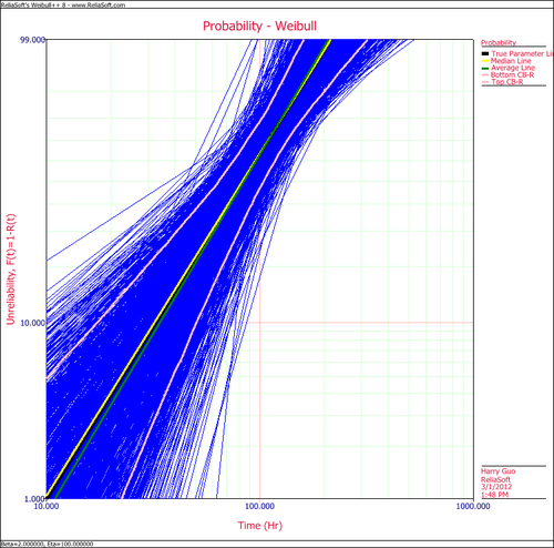
The following plot shows the simulation-based confidence bounds for the RRX parameter estimation method, as well as the expected variation due to sampling error. | The following plot shows the simulation-based confidence bounds for the RRX parameter estimation method, as well as the expected variation due to sampling error. | ||
[[Image:SimuMatic RRX.png|center|500px|'''RRX''']] | [[Image:SimuMatic RRX.png|center|500px|'''RRX''']] | ||
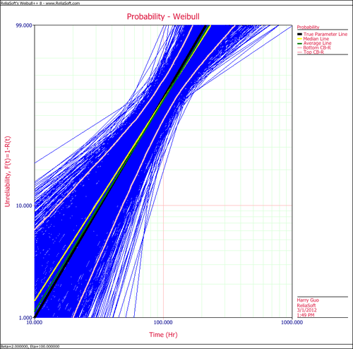
Create another SimuMatic folio and generate a second data using the same settings, but this time, select the RRY analysis method on the Analysis tab. The following plot shows the result. | Create another SimuMatic folio and generate a second data using the same settings, but this time, select the RRY analysis method on the Analysis tab. The following plot shows the result. | ||
[[Image:SimuMatic RRY.png|center|500px|'''RRY''']] | [[Image:SimuMatic RRY.png|center|500px|'''RRY''']] | ||
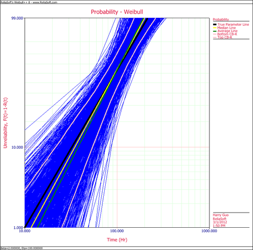
The following plot shows the results using the MLE analysis method. | The following plot shows the results using the MLE analysis method. | ||
[[Image:SimuMatic MLE.png|center|500px|'''MLE''']] | [[Image:SimuMatic MLE.png|center|500px|'''MLE''']] | ||
The results clearly demonstrate that the median RRX estimate provides the least deviation from the truth for this sample size and data type. However, the MLE outputs are grouped more closely together, as evidenced by the bounds. | The results clearly demonstrate that the median RRX estimate provides the least deviation from the truth for this sample size and data type. However, the MLE outputs are grouped more closely together, as evidenced by the bounds. | ||
This experiment can be repeated in SimuMatic using multiple censoring schemes (including Type I and Type II right censoring as well as random censoring) with various distributions. Multiple experiments can be performed with this utility to evaluate assumptions about the appropriate parameter estimation method to use for data sets. | This experiment can be repeated in SimuMatic using multiple censoring schemes (including Type I and Type II right censoring as well as random censoring) with various distributions. Multiple experiments can be performed with this utility to evaluate assumptions about the appropriate parameter estimation method to use for data sets. | ||
Latest revision as of 18:58, 18 September 2023
New format available! This reference is now available in a new format that offers faster page load, improved display for calculations and images and more targeted search.
As of January 2024, this Reliawiki page will not continue to be updated. Please update all links and bookmarks to the latest references at Weibull examples and Weibull reference examples.
This example appears in the Life data analysis reference and Accelerated life testing reference.
Comparing Parameter Estimation Methods Using Simulation Based Bounds
The purpose of this example is to determine the best parameter estimation method for a sample of ten units with complete time-to-failure data for each unit (i.e., no censoring). The data set follows a Weibull distribution with [math]\displaystyle{ \beta =2\,\! }[/math] and [math]\displaystyle{ \eta =100\,\! }[/math] hours.
The confidence bounds for the data set could be obtained by using Weibull++'s SimuMatic utility. To obtain the results, use the following settings in SimuMatic.
- On the Main tab, choose the 2P-Weibull distribution and enter the given parameters (i.e., [math]\displaystyle{ \beta =2\,\! }[/math] and [math]\displaystyle{ \eta =100\,\! }[/math] hours)
- On the Censoring tab, select the No censoring option.
- On the Settings tab, set the number of data sets to 1,000 and the number of data points to 10.
- On the Analysis tab, choose the RRX analysis method and set the confidence bounds to 90.
The following plot shows the simulation-based confidence bounds for the RRX parameter estimation method, as well as the expected variation due to sampling error.
Create another SimuMatic folio and generate a second data using the same settings, but this time, select the RRY analysis method on the Analysis tab. The following plot shows the result.
The following plot shows the results using the MLE analysis method.
The results clearly demonstrate that the median RRX estimate provides the least deviation from the truth for this sample size and data type. However, the MLE outputs are grouped more closely together, as evidenced by the bounds.
This experiment can be repeated in SimuMatic using multiple censoring schemes (including Type I and Type II right censoring as well as random censoring) with various distributions. Multiple experiments can be performed with this utility to evaluate assumptions about the appropriate parameter estimation method to use for data sets.


