Non Parametric RDA MCF Example: Difference between revisions
Kate Racaza (talk | contribs) No edit summary |
Lisa Hacker (talk | contribs) No edit summary |
||
| (13 intermediate revisions by 5 users not shown) | |||
| Line 1: | Line 1: | ||
<noinclude>{{Banner Weibull Examples}} | <noinclude>{{Banner Weibull Examples}} | ||
''This | ''This example appears in the [https://help.reliasoft.com/reference/life_data_analysis Life data analysis reference].'' | ||
</noinclude> | </noinclude> | ||
| Line 13: | Line 13: | ||
\text{4} & \text{13, 15, 24+} \\ | \text{4} & \text{13, 15, 24+} \\ | ||
\text{5} & \text{16, 22, 25, 28+} \\ | \text{5} & \text{16, 22, 25, 28+} \\ | ||
\end{matrix}</math></center> | \end{matrix}\,\!</math></center> | ||
Estimate the MCF values, with 95% confidence bounds. | Estimate the MCF values, with 95% confidence bounds. | ||
| Line 28: | Line 28: | ||
\text{1} & \text{10} & \text{F} & \text{5} & \text{0}\text{.20} & \text{0}\text{.40 + 0}\text{.20 = 0}\text{.60} \\ | \text{1} & \text{10} & \text{F} & \text{5} & \text{0}\text{.20} & \text{0}\text{.40 + 0}\text{.20 = 0}\text{.60} \\ | ||
\text{3} & \text{12} & \text{F} & \text{5} & \text{0}\text{.20} & \text{0}\text{.60 + 0}\text{.20 = 0}\text{.80} \\ | \text{3} & \text{12} & \text{F} & \text{5} & \text{0}\text{.20} & \text{0}\text{.60 + 0}\text{.20 = 0}\text{.80} \\ | ||
\text{2} & \text{13} & \text{F} & \text{5} & \text{0}\text{.20} & \text{0}\text{.80+0}\text{.20 =1}\text{.00} \\ | \text{2} & \text{13} & \text{F} & \text{5} & \text{0}\text{.20} & \text{0}\text{.80 + 0}\text{.20 = 1}\text{.00} \\ | ||
\text{4} & \text{13} & \text{F} & \text{5} & \text{0}\text{.20} & \text{1}\text{.00 + 0}\text{.20 = 1}\text{.20} \\ | \text{4} & \text{13} & \text{F} & \text{5} & \text{0}\text{.20} & \text{1}\text{.00 + 0}\text{.20 = 1}\text{.20} \\ | ||
\text{1} & \text{15} & \text{F} & \text{5} & \text{0}\text{.20} & \text{1}\text{.20 + 0}\text{.20 =1}\text{.40} \\ | \text{1} & \text{15} & \text{F} & \text{5} & \text{0}\text{.20} & \text{1}\text{.20 + 0}\text{.20 = 1}\text{.40} \\ | ||
\text{4} & \text{15} & \text{F} & \text{5} & \text{0}\text{.20} & \text{1}\text{.40 + 0}\text{.20 = 1}\text{.60} \\ | \text{4} & \text{15} & \text{F} & \text{5} & \text{0}\text{.20} & \text{1}\text{.40 + 0}\text{.20 = 1}\text{.60} \\ | ||
\text{5} & \text{16} & \text{F} & \text{5} & \text{0}\text{.20} & \text{1}\text{.60 + 0}\text{.20 = 1}\text{.80} \\ | \text{5} & \text{16} & \text{F} & \text{5} & \text{0}\text{.20} & \text{1}\text{.60 + 0}\text{.20 = 1}\text{.80} \\ | ||
\text{2} & \text{17} & \text{F} & \text{5} & \text{0}\text{.20} & \text{1}\text{.80 + 0}\text{.20 = 2}\text{. | \text{2} & \text{17} & \text{F} & \text{5} & \text{0}\text{.20} & \text{1}\text{.80 + 0}\text{.20 = 2}\text{.00} \\ | ||
\text{1} & \text{17} & \text{S} & \text{4} & {} & {} \\ | \text{1} & \text{17} & \text{S} & \text{4} & {} & {} \\ | ||
\text{2} & \text{19} & \text{S} & \text{3} & {} & {} \\ | \text{2} & \text{19} & \text{S} & \text{3} & {} & {} \\ | ||
| Line 43: | Line 43: | ||
\text{3} & \text{26} & \text{S} & \text{1} & {} & {} \\ | \text{3} & \text{26} & \text{S} & \text{1} & {} & {} \\ | ||
\text{5} & \text{28} & \text{S} & \text{0} & {} & {} \\ | \text{5} & \text{28} & \text{S} & \text{0} & {} & {} \\ | ||
\end{matrix}</math></center> | \end{matrix}\,\!</math></center> | ||
Using the MCF variance equation, the following table of variance values can be obtained: | Using the MCF variance equation, the following table of variance values can be obtained: | ||
| Line 52: | Line 52: | ||
! Months | ! Months | ||
! State | ! State | ||
! < | ! <math>{{r}_{i}}\,\!</math> | ||
! < | ! <math>Va{{r}_{i}}\,\!</math> | ||
|- | |- | ||
| 1 | | 1 | ||
| Line 59: | Line 59: | ||
| F | | F | ||
| 5 | | 5 | ||
| <math>(\tfrac{1}{5})^2[(1-\tfrac{1}{5})^2+4(0-\tfrac{1}{5})^2]=0.032</math> | | <math>(\tfrac{1}{5})^2[(1-\tfrac{1}{5})^2+4(0-\tfrac{1}{5})^2]=0.032\,\!</math> | ||
|- | |- | ||
| 2 | | 2 | ||
| Line 65: | Line 65: | ||
| F | | F | ||
| 5 | | 5 | ||
| <math>0.032+(\tfrac{1}{5})^2[(1-\tfrac{1}{5})^2+4(0-\tfrac{1}{5})^2]=0.064</math> | | <math>0.032+(\tfrac{1}{5})^2[(1-\tfrac{1}{5})^2+4(0-\tfrac{1}{5})^2]=0.064\,\!</math> | ||
|- | |- | ||
| 1 | | 1 | ||
| Line 71: | Line 71: | ||
| F | | F | ||
| 5 | | 5 | ||
| <math>0.064+(\tfrac{1}{5})^2[(1-\tfrac{1}{5})^2+4(0-\tfrac{1}{5})^2]=0.096</math> | | <math>0.064+(\tfrac{1}{5})^2[(1-\tfrac{1}{5})^2+4(0-\tfrac{1}{5})^2]=0.096\,\!</math> | ||
|- | |- | ||
| 3 | | 3 | ||
| Line 77: | Line 77: | ||
| F | | F | ||
| 5 | | 5 | ||
| <math>0.096+(\tfrac{1}{5})^2[(1-\tfrac{1}{5})^2+4(0-\tfrac{1}{5})^2]=0.128</math> | | <math>0.096+(\tfrac{1}{5})^2[(1-\tfrac{1}{5})^2+4(0-\tfrac{1}{5})^2]=0.128\,\!</math> | ||
|- | |- | ||
| 2 | | 2 | ||
| Line 83: | Line 83: | ||
| F | | F | ||
| 5 | | 5 | ||
| <math>0.128+(\tfrac{1}{5})^2[(1-\tfrac{1}{5})^2+4(0-\tfrac{1}{5})^2]=0.160</math> | | <math>0.128+(\tfrac{1}{5})^2[(1-\tfrac{1}{5})^2+4(0-\tfrac{1}{5})^2]=0.160\,\!</math> | ||
|- | |- | ||
| 4 | | 4 | ||
| Line 89: | Line 89: | ||
| F | | F | ||
| 5 | | 5 | ||
| <math>0.160+(\tfrac{1}{5})^2[(1-\tfrac{1}{5})^2+4(0-\tfrac{1}{5})^2]=0.192</math> | | <math>0.160+(\tfrac{1}{5})^2[(1-\tfrac{1}{5})^2+4(0-\tfrac{1}{5})^2]=0.192\,\!</math> | ||
|- | |- | ||
| 1 | | 1 | ||
| Line 95: | Line 95: | ||
| F | | F | ||
| 5 | | 5 | ||
| <math>0.192+(\tfrac{1}{5})^2[(1-\tfrac{1}{5})^2+4(0-\tfrac{1}{5})^2]=0.224</math> | | <math>0.192+(\tfrac{1}{5})^2[(1-\tfrac{1}{5})^2+4(0-\tfrac{1}{5})^2]=0.224\,\!</math> | ||
|- | |- | ||
| 4 | | 4 | ||
| Line 101: | Line 101: | ||
| F | | F | ||
| 5 | | 5 | ||
| <math>0.224+(\tfrac{1}{5})^2[(1-\tfrac{1}{5})^2+4(0-\tfrac{1}{5})^2]=0.256</math> | | <math>0.224+(\tfrac{1}{5})^2[(1-\tfrac{1}{5})^2+4(0-\tfrac{1}{5})^2]=0.256\,\!</math> | ||
|- | |- | ||
| 5 | | 5 | ||
| Line 107: | Line 107: | ||
| F | | F | ||
| 5 | | 5 | ||
| <math>0.256+(\tfrac{1}{5})^2[ | | <math>0.256+(\tfrac{1}{5})^2[(1-\tfrac{1}{5})^2+4(0-\tfrac{1}{5})^2]=0.288\,\!</math> | ||
|- | |- | ||
| 2 | | 2 | ||
| Line 113: | Line 113: | ||
| F | | F | ||
| 5 | | 5 | ||
| <math>0.288+(\tfrac{1}{5})^2[(1-\tfrac{1}{5})^2+4(0-\tfrac{1}{5})^2]=0.320</math> | | <math>0.288+(\tfrac{1}{5})^2[(1-\tfrac{1}{5})^2+4(0-\tfrac{1}{5})^2]=0.320\,\!</math> | ||
|- | |- | ||
| 1 | | 1 | ||
| Line 131: | Line 131: | ||
| F | | F | ||
| 3 | | 3 | ||
| <math>0.320+(\tfrac{1}{ | | <math>0.320+(\tfrac{1}{3})^2[(1-\tfrac{1}{3})^2+2(0-\tfrac{1}{3})^2]=0.394\,\!</math> | ||
|- | |- | ||
| 5 | | 5 | ||
| Line 137: | Line 137: | ||
| F | | F | ||
| 3 | | 3 | ||
| <math>0.394+(\tfrac{1}{ | | <math>0.394+(\tfrac{1}{3})^2[(1-\tfrac{1}{3})^2+2(0-\tfrac{1}{3})^2]=0.468\,\!</math> | ||
|- | |- | ||
| 4 | | 4 | ||
| Line 149: | Line 149: | ||
| F | | F | ||
| 2 | | 2 | ||
| <math>0.468+(\tfrac{1}{ | | <math>0.468+(\tfrac{1}{2})^2[(1-\tfrac{1}{2})^2+(0-\tfrac{1}{2})^2]=0.593\,\!</math> | ||
|- | |- | ||
| 5 | | 5 | ||
| Line 155: | Line 155: | ||
| F | | F | ||
| 2 | | 2 | ||
| <math>0. | | <math>0.593+(\tfrac{1}{2})^2[(1-\tfrac{1}{2})^2+(0-\tfrac{1}{2})^2]=0.718\,\!</math> | ||
|- | |- | ||
| 3 | | 3 | ||
| Line 170: | Line 170: | ||
|} | |} | ||
Using the equation for the MCF bounds and < | Using the equation for the MCF bounds and <math>{{K}_{5}} = 1.644\,\!</math> for a 95% confidence level, the confidence bounds can be obtained as follows: | ||
<center><math>\begin{matrix} | <center><math>\begin{matrix} | ||
| Line 183: | Line 183: | ||
\text{4} & \text{15} & \text{F} & \text{1}\text{.60} & \text{0}\text{.256} & 0.9511 & 2.6916 \\ | \text{4} & \text{15} & \text{F} & \text{1}\text{.60} & \text{0}\text{.256} & 0.9511 & 2.6916 \\ | ||
\text{5} & \text{16} & \text{F} & \text{1}\text{.80} & \text{0}\text{.288} & 1.1023 & 2.9393 \\ | \text{5} & \text{16} & \text{F} & \text{1}\text{.80} & \text{0}\text{.288} & 1.1023 & 2.9393 \\ | ||
\text{2} & \text{17} & \text{F} & \text{2}\text{. | \text{2} & \text{17} & \text{F} & \text{2}\text{.00} & \text{0}\text{.320} & 1.2560 & 3.1848 \\ | ||
\text{1} & \text{17} & \text{S} & {} & {} & {} & {} \\ | \text{1} & \text{17} & \text{S} & {} & {} & {} & {} \\ | ||
\text{2} & \text{19} & \text{S} & {} & {} & {} & {} \\ | \text{2} & \text{19} & \text{S} & {} & {} & {} & {} \\ | ||
| Line 193: | Line 193: | ||
\text{3} & \text{26} & \text{S} & {} & {} & {} & {} \\ | \text{3} & \text{26} & \text{S} & {} & {} & {} & {} \\ | ||
\text{5} & \text{28} & \text{S} & {} & {} & {} & {} \\ | \text{5} & \text{28} & \text{S} & {} & {} & {} & {} \\ | ||
\end{matrix}</math></center> | \end{matrix}\,\!</math></center> | ||
The analysis presented in this example can be performed automatically in Weibull++'s non-parametric RDA folio, as shown next. | The analysis presented in this example can be performed automatically in Weibull++'s non-parametric RDA folio, as shown next. | ||
[[Image:Recurrent Data Example 2 Data.png|center| | [[Image:Recurrent Data Example 2 Data.png|center|650px]] | ||
Note: In the folio above, the < | Note: In the folio above, the <math>F\,\!</math> refers to failures and <math>E\,\!</math> refers to suspensions (or censoring ages). The results, with calculated MCF values and upper and lower 95% confidence limits, are shown next along with the graphical plot. | ||
[[Image:Recurrent Data Example 2 Result.png|center| | [[Image:Recurrent Data Example 2 Result.png|center|650px]] | ||
[[Image:Recurrent Data Example 2 Plot.png|center|550px]] | [[Image:Recurrent Data Example 2 Plot.png|center|550px]] | ||
Latest revision as of 18:53, 18 September 2023
New format available! This reference is now available in a new format that offers faster page load, improved display for calculations and images and more targeted search.
As of January 2024, this Reliawiki page will not continue to be updated. Please update all links and bookmarks to the latest references at Weibull examples and Weibull reference examples.
This example appears in the Life data analysis reference.
A health care company maintains five identical pieces of equipment used by a hospital. When a piece of equipment fails, the company sends a crew to repair it. The following table gives the failure and censoring ages for each machine, where the + sign indicates a censoring age.
Estimate the MCF values, with 95% confidence bounds.
Solution
The MCF estimates are obtained as follows:
Using the MCF variance equation, the following table of variance values can be obtained:
| ID | Months | State | [math]\displaystyle{ {{r}_{i}}\,\! }[/math] | [math]\displaystyle{ Va{{r}_{i}}\,\! }[/math] |
|---|---|---|---|---|
| 1 | 5 | F | 5 | [math]\displaystyle{ (\tfrac{1}{5})^2[(1-\tfrac{1}{5})^2+4(0-\tfrac{1}{5})^2]=0.032\,\! }[/math] |
| 2 | 6 | F | 5 | [math]\displaystyle{ 0.032+(\tfrac{1}{5})^2[(1-\tfrac{1}{5})^2+4(0-\tfrac{1}{5})^2]=0.064\,\! }[/math] |
| 1 | 10 | F | 5 | [math]\displaystyle{ 0.064+(\tfrac{1}{5})^2[(1-\tfrac{1}{5})^2+4(0-\tfrac{1}{5})^2]=0.096\,\! }[/math] |
| 3 | 12 | F | 5 | [math]\displaystyle{ 0.096+(\tfrac{1}{5})^2[(1-\tfrac{1}{5})^2+4(0-\tfrac{1}{5})^2]=0.128\,\! }[/math] |
| 2 | 13 | F | 5 | [math]\displaystyle{ 0.128+(\tfrac{1}{5})^2[(1-\tfrac{1}{5})^2+4(0-\tfrac{1}{5})^2]=0.160\,\! }[/math] |
| 4 | 13 | F | 5 | [math]\displaystyle{ 0.160+(\tfrac{1}{5})^2[(1-\tfrac{1}{5})^2+4(0-\tfrac{1}{5})^2]=0.192\,\! }[/math] |
| 1 | 15 | F | 5 | [math]\displaystyle{ 0.192+(\tfrac{1}{5})^2[(1-\tfrac{1}{5})^2+4(0-\tfrac{1}{5})^2]=0.224\,\! }[/math] |
| 4 | 15 | F | 5 | [math]\displaystyle{ 0.224+(\tfrac{1}{5})^2[(1-\tfrac{1}{5})^2+4(0-\tfrac{1}{5})^2]=0.256\,\! }[/math] |
| 5 | 16 | F | 5 | [math]\displaystyle{ 0.256+(\tfrac{1}{5})^2[(1-\tfrac{1}{5})^2+4(0-\tfrac{1}{5})^2]=0.288\,\! }[/math] |
| 2 | 17 | F | 5 | [math]\displaystyle{ 0.288+(\tfrac{1}{5})^2[(1-\tfrac{1}{5})^2+4(0-\tfrac{1}{5})^2]=0.320\,\! }[/math] |
| 1 | 17 | S | 4 | |
| 2 | 19 | S | 3 | |
| 3 | 20 | F | 3 | [math]\displaystyle{ 0.320+(\tfrac{1}{3})^2[(1-\tfrac{1}{3})^2+2(0-\tfrac{1}{3})^2]=0.394\,\! }[/math] |
| 5 | 22 | F | 3 | [math]\displaystyle{ 0.394+(\tfrac{1}{3})^2[(1-\tfrac{1}{3})^2+2(0-\tfrac{1}{3})^2]=0.468\,\! }[/math] |
| 4 | 24 | S | 2 | |
| 3 | 25 | F | 2 | [math]\displaystyle{ 0.468+(\tfrac{1}{2})^2[(1-\tfrac{1}{2})^2+(0-\tfrac{1}{2})^2]=0.593\,\! }[/math] |
| 5 | 25 | F | 2 | [math]\displaystyle{ 0.593+(\tfrac{1}{2})^2[(1-\tfrac{1}{2})^2+(0-\tfrac{1}{2})^2]=0.718\,\! }[/math] |
| 3 | 26 | S | 1 | |
| 5 | 28 | S | 0 |
Using the equation for the MCF bounds and [math]\displaystyle{ {{K}_{5}} = 1.644\,\! }[/math] for a 95% confidence level, the confidence bounds can be obtained as follows:
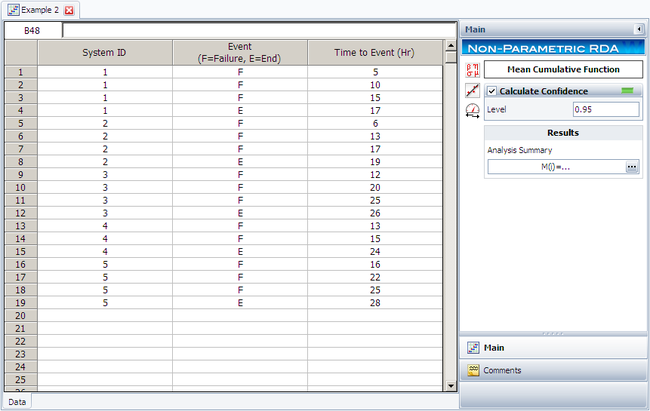
The analysis presented in this example can be performed automatically in Weibull++'s non-parametric RDA folio, as shown next.
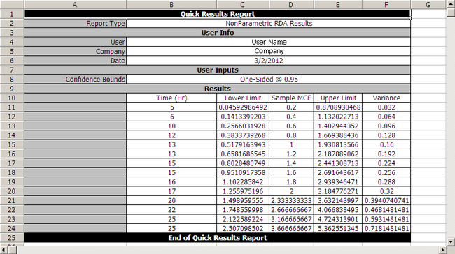
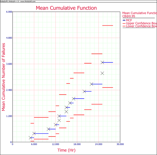
Note: In the folio above, the [math]\displaystyle{ F\,\! }[/math] refers to failures and [math]\displaystyle{ E\,\! }[/math] refers to suspensions (or censoring ages). The results, with calculated MCF values and upper and lower 95% confidence limits, are shown next along with the graphical plot.


