Example: Parametric RDA - Air Condition Unit: Difference between revisions
Kate Racaza (talk | contribs) (proofread) |
Lisa Hacker (talk | contribs) No edit summary |
||
| (10 intermediate revisions by 3 users not shown) | |||
| Line 1: | Line 1: | ||
{{Banner Weibull Examples}} | <noinclude>{{Banner Weibull Examples}} | ||
''This example appears in the [https://help.reliasoft.com/reference/life_data_analysis Life data analysis reference]''. | |||
</noinclude>The following table gives the failure times for the air conditioning unit of an aircraft. The observation ended by the time the last failure occurred, as discussed in Cox [[Appendix:_Life_Data_Analysis_References|[3]]]. | |||
<center><math>\begin{matrix} | <center><math>\begin{matrix} | ||
| Line 10: | Line 10: | ||
\text{268} & \text{544} & \text{950} & \text{1362} & \text{1539} \\ | \text{268} & \text{544} & \text{950} & \text{1362} & \text{1539} \\ | ||
\text{290} & \text{732} & \text{955} & \text{1459} & {} \\ | \text{290} & \text{732} & \text{955} & \text{1459} & {} \\ | ||
\end{matrix}</math></center> | \end{matrix}\,\!</math></center> | ||
1. Estimate the GRP model parameters using the Type I virtual age option. | 1. Estimate the GRP model parameters using the Type I virtual age option. | ||
| Line 21: | Line 20: | ||
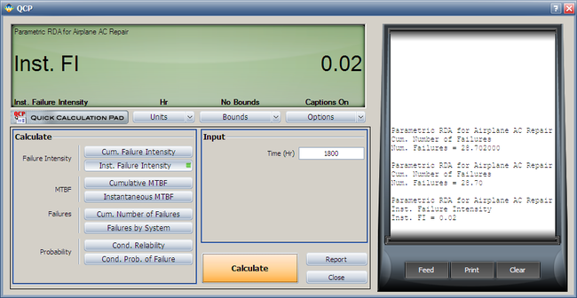
4. Using the QCP, calculate the expected failure number and expected instantaneous failure intensity by time 1800. | 4. Using the QCP, calculate the expected failure number and expected instantaneous failure intensity by time 1800. | ||
'''Solution''' | |||
Enter the data into a parametric RDA folio in Weibull++. On the control panel, select the '''3''' parameters option and the '''Type I''' setting. Keep the default simulation settings. Click '''Calculate'''. | Enter the data into a parametric RDA folio in Weibull++. On the control panel, select the '''3''' parameters option and the '''Type I''' setting. Keep the default simulation settings. Click '''Calculate'''. | ||
:1. The estimated parameters are <math>\hat{\beta }=1.1976\,\!</math>, <math>\hat{\lambda }=4.94E-03\,\!</math>, <math>\hat{q}=0.1344\,\!</math>. | |||
:1. The estimated parameters are <math>\hat{\beta }=1.1976,</math> <math>\hat{\lambda }=4.94E-03,</math> <math>\hat{q}=0.1344</math> . | |||
:2. The following plots show the cumulative number of failures and instantaneous failure intensity, respectively. | :2. The following plots show the cumulative number of failures and instantaneous failure intensity, respectively. | ||
[[Image:Parametric RDA N(T) plot.png|center|650px]] | |||
[[Image:Parametric RDA Lambda(T) plot.png|center|650px]] | |||
:3. The following plot shows the conditional reliability. | :3. The following plot shows the conditional reliability. | ||
[[Image:Parametric RDA Cond R(T) plot.png | [[Image:Parametric RDA Cond R(T) plot.png|center|650px]] | ||
:4. Using the QCP, the failure number and instantaneous failure intensity are: | :4. Using the QCP, the failure number and instantaneous failure intensity are: | ||
[[Image:QCP N(T).png | [[Image:QCP N(T).png|center|650px]] | ||
[[Image:QCP Lambda(T).png | [[Image:QCP Lambda(T).png|center|650px]] | ||
Latest revision as of 18:52, 18 September 2023
New format available! This reference is now available in a new format that offers faster page load, improved display for calculations and images and more targeted search.
As of January 2024, this Reliawiki page will not continue to be updated. Please update all links and bookmarks to the latest references at Weibull examples and Weibull reference examples.
This example appears in the Life data analysis reference.
The following table gives the failure times for the air conditioning unit of an aircraft. The observation ended by the time the last failure occurred, as discussed in Cox [3].
1. Estimate the GRP model parameters using the Type I virtual age option.
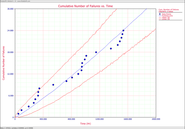
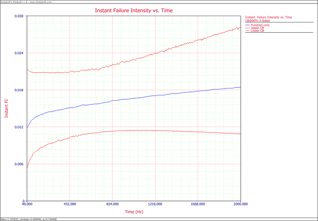
2. Plot the failure number and instantaneous failure intensity vs. time with 90% two-sided confidence bounds.
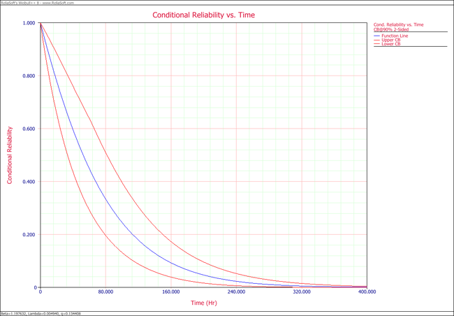
3. Plot the conditional reliability vs. time with 90% two-sided confidence bounds. The mission start time is 40 and mission time is varying.
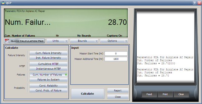
4. Using the QCP, calculate the expected failure number and expected instantaneous failure intensity by time 1800.
Solution
Enter the data into a parametric RDA folio in Weibull++. On the control panel, select the 3 parameters option and the Type I setting. Keep the default simulation settings. Click Calculate.
- 1. The estimated parameters are [math]\displaystyle{ \hat{\beta }=1.1976\,\! }[/math], [math]\displaystyle{ \hat{\lambda }=4.94E-03\,\! }[/math], [math]\displaystyle{ \hat{q}=0.1344\,\! }[/math].
- 2. The following plots show the cumulative number of failures and instantaneous failure intensity, respectively.
- 3. The following plot shows the conditional reliability.
- 4. Using the QCP, the failure number and instantaneous failure intensity are:

